FAQ
AutoResp™ error message "No boards have been configured"
When starting AutoResp™ and this error message appear, AutoResp™ was not installed with administrator rights. During the AutoResp™ installation process, a file must be copied into a Windows system folder. This requires an administrator login. Here is the instruction how to install the necessary file to get rid of the error message:
- Login as an administrator
- Download the following configuration file (LINK) and save the file to your desktop.
- Locate the folder folder: C:\ProgramData\Measurement Computing\DAQ\ . The folder Program Data is a system hidden folder. So you might have to change settings for the folder in order see hidden folders and system files. Hidden folders are shown as “transparent” in Windows’ file explorer.
- If the folder doesnt exist, please create it.
- Now move the file into this folder.
- After you moved the file, change folder settings again to hide hidden and system files.
- Start AutoResp™. The error message should be gone by now.
OXY-REG error message "SE.BR"?
If the display on your OXY-REG is giving the error message "SE.BR" (sensor breakage), it means that the signal input type for the instrument has been changed from the default setting (potmeter).
To change the input type back to the default setting, press the OK button once. Then press the arrow buttons until the input type POTM (potmeter) is shown in the display and then press OK to choose this. Finally exit the set up menu by pressing the OK button several times until the display shows - - - -.
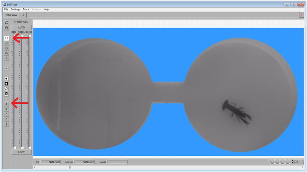
How to draw zones/masks in LoliTrack 4 and ShuttleSoft 1?
This guide shows you how to draw zones and mask in LoliTrack and ShuttleSoft.
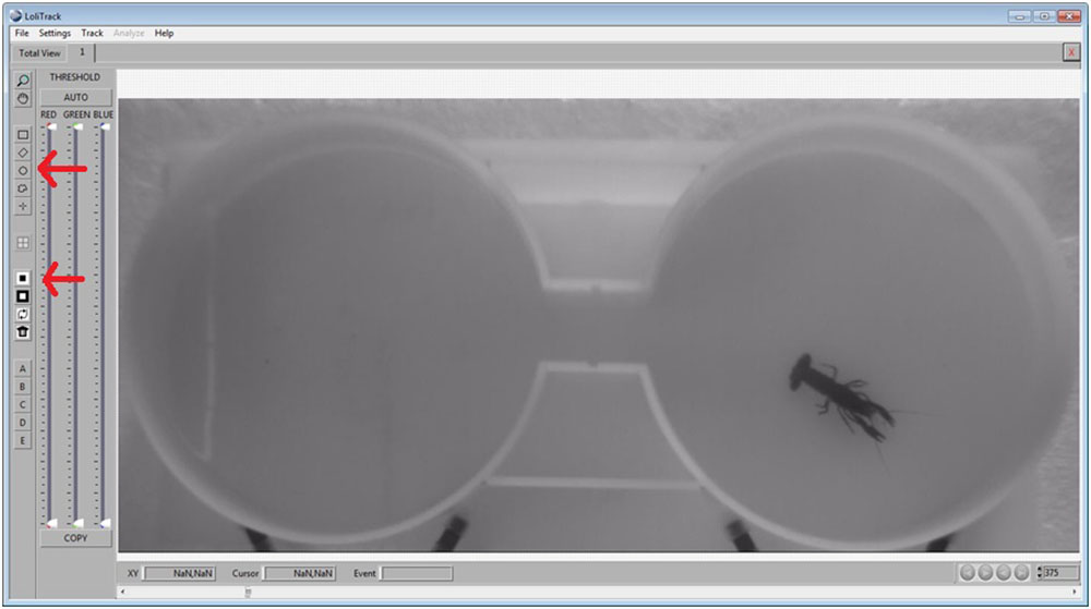
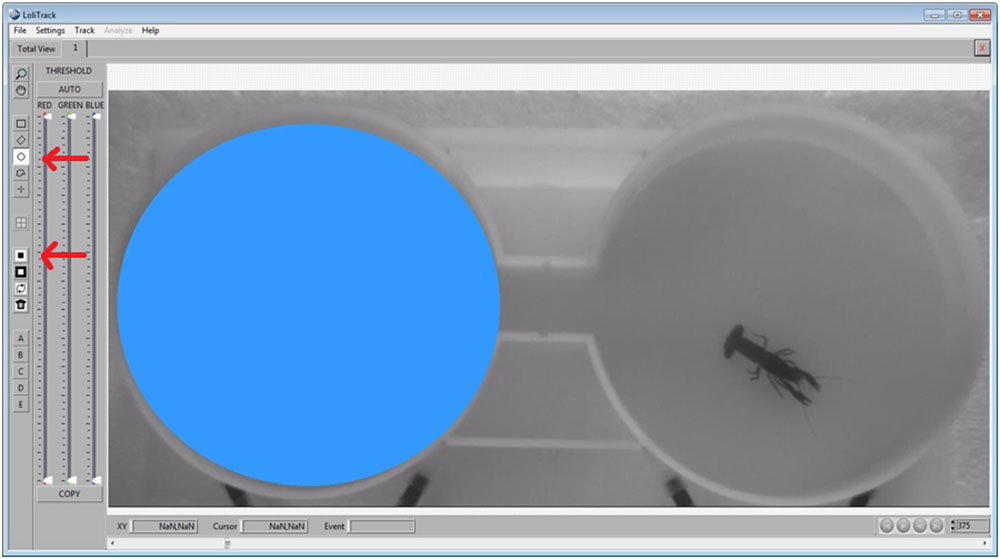
Use the Circle button, then draw a circle in one of the compartments. Afterwards, click on the Mask Inside Area button.
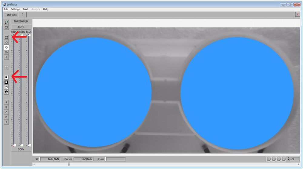
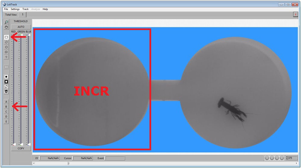
Use the Circle button again to draw a circle in the other compartment. Afterwards, click on the Mask Inside Area button.
Use the Rectangular button, then draw a rectangle between the two compartments. Afterwards, click on the Mask Inside Area button.
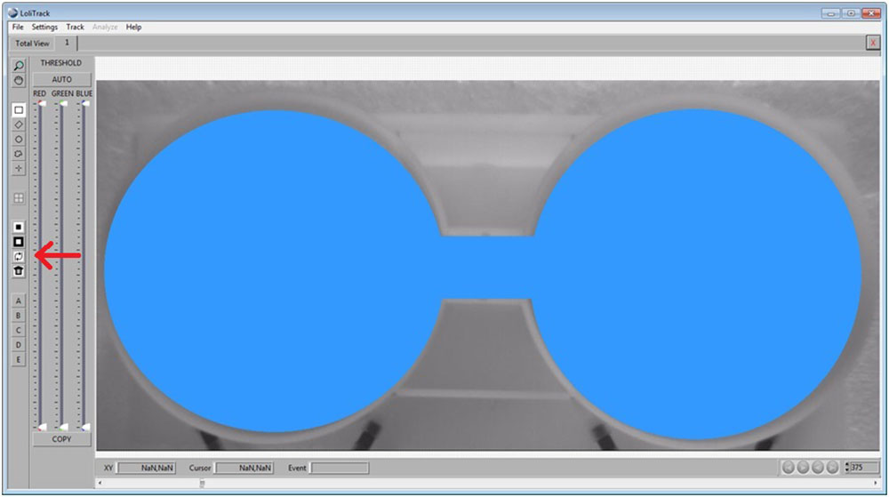
Now invert the mask by clicking on the Invert Mask button.
Draw a rectangular area in one compartment, and click on a Zone button (A, B, C...). This area is now defined as a zone of interest.
Draw a rectangular area in the other compartment, and click on a different Zone button. This area is now also defined as a zone of interest.
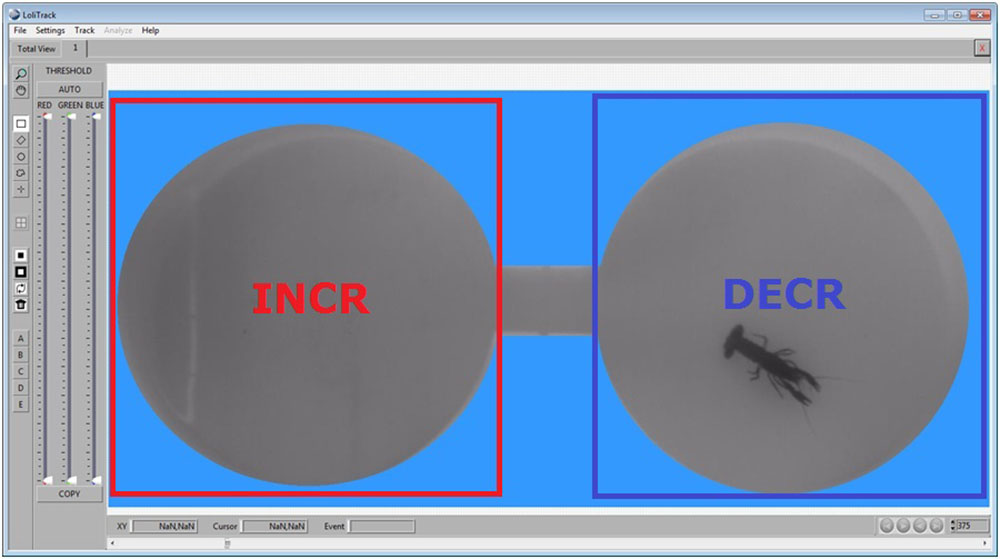
This is an example of how a typical mask and zones could look like running a ShuttleSoft experiment.
LinkWhy is the PIT reader software in German?
To change the language in the PIT tag reader software (APR-PC-DEMO) from German to English, please go to the following program files folder on your PC:
- Locate C:\Program Files (x86)\AgriDent
- Delete the file(s) that has the *.lng file extension (e.g. Agrident.lng).
- Without this language file, the software will now use the default language (English).
What type of oxygen sensor should I use?
Loligo® Systems offers the three main types of oxygen sensors differing in measuring principle, response time, sensor size, maintenance requirement and pricing.
1. Optical oxygen sensors
For many invasive techniques, measurements in tiny volumes (e.g. micro respirometry) or applications which require high temporal and spatial resolution, fibre-optic oxygen sensors are the only solution.
Even for general purposes we recommend optical oxygen sensors featuring low maintenance requirements, high stability and accuracy, no electrical interference, no ground loop problems, and zero O2 consumption by the sensor.
The main disadvantages is price, single-channel meters start at about €3750. A high temperature sensitivity of this technology and a fragile tip on the <50-140 nm micro sensors might also be a problem in some applications. The macro sensors, on the other hand, are very tough.
2. Galvanic cell oxygen electrodes
Galvanic type oxygen probes are inexpensive and rugged sensors producing a milliVolt signal for easy instrumentation without supplying power.
We recommend galvanic probes for applications like respirometry and field measurements, and as a low-budget alternative to optical oxygen equipment, e.g. for multi-channel systems. They can be used with relatively long cables (+25 meters). We recommend using a galvanic isolation preamplifier between the probe and any data acquisition system to minimize possible ground loop problems.
The main disadvantage of galvanic probes is a relative long response time and oxygen self-consumption making them unsuitable for measurements in small volumes and in un-mixed samples.
3. Polarographic oxygen electrodes (or Clark type electrodes)
Low oxygen self-consumption and a small size make these sensors suitable for physiological setups like blood gas analysis and low volume respirometry.
However, Clark type electrodes require much maintenance, often membranes and electrolyte fluid should be changed on a daily basis, and polarographic amplifiers for these sensors are quite costly.
Thus, we recommend the E101 as a replacement oxygen electrode for customers with their own polarograhic oxygen meter, e.g. PHM meter from Radiometer Copenhagen, OM200 from Cameron Instr. Co. etc.
LinkHow to calibrate an oxygen sensor?
CALIBRATION PRINCIPLE
Instrument calibration is an essential first step in analytical and measurement procedures. The rationale for a two-point calibration is to provide two points of reference with which to calibrate the instrument and, therefore, ensuring accurate measurements with your sensor of the unknown concentrations of your samples. A two-point calibration between two extremes are advocated, e.g. 0 - 100 % air saturation. For the low calibration point, we recommend using either nitrogen gas or sodium sulphite solution, for the high calibration point, bubble atmospheric air using an aerator. Please see below for general step-wise instructions on how to carry out a two point calibration. For specific instructions for a particular oxygen instrument, please click on the specific links.
GENERAL
- Connect the probe to the oxygen instrument and turn on the instrument.
- Place the tip of the probe in a mixed air-equilibrated water sample. This can be achived by purging atmospheric air into sample water, e.g. with an air pump and air stone.
- Wait for the reading to stabilize. Then save this point as the HIGH calibration value (100% air saturation).
- Place the tip of the probe in an oxygen free water sample (e.g. by purging nitrogen gas into sample water or by dissolving ~10 grams of Na2SO3 in 500 mL of distilled water).
- Wait for the reading to stabilize. Then save this point as the LOW calibration value (0% air saturation).
- Rinse the probe with distilled water.
- Place the probe into the sample, and record the sample oxygen saturation when the reading is stable.
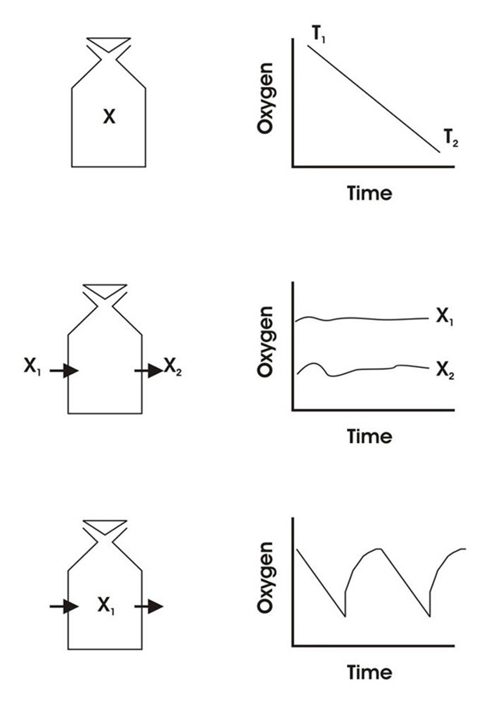
See below for a diagrammatic representation of sensor readings at:
- 100 % to 0 % air saturation
- 0 % to 100 % air saturation
- 100 % to 0 % and back up to 100 % air saturation.
 |
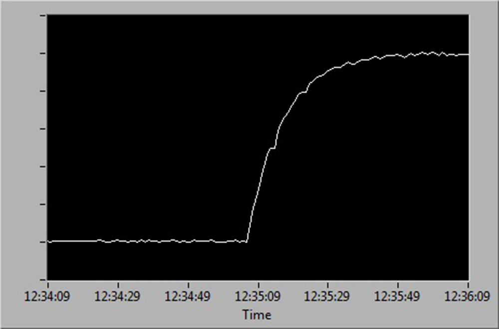 |
| 100% to 0% air saturation | 0% to 100% air saturation |
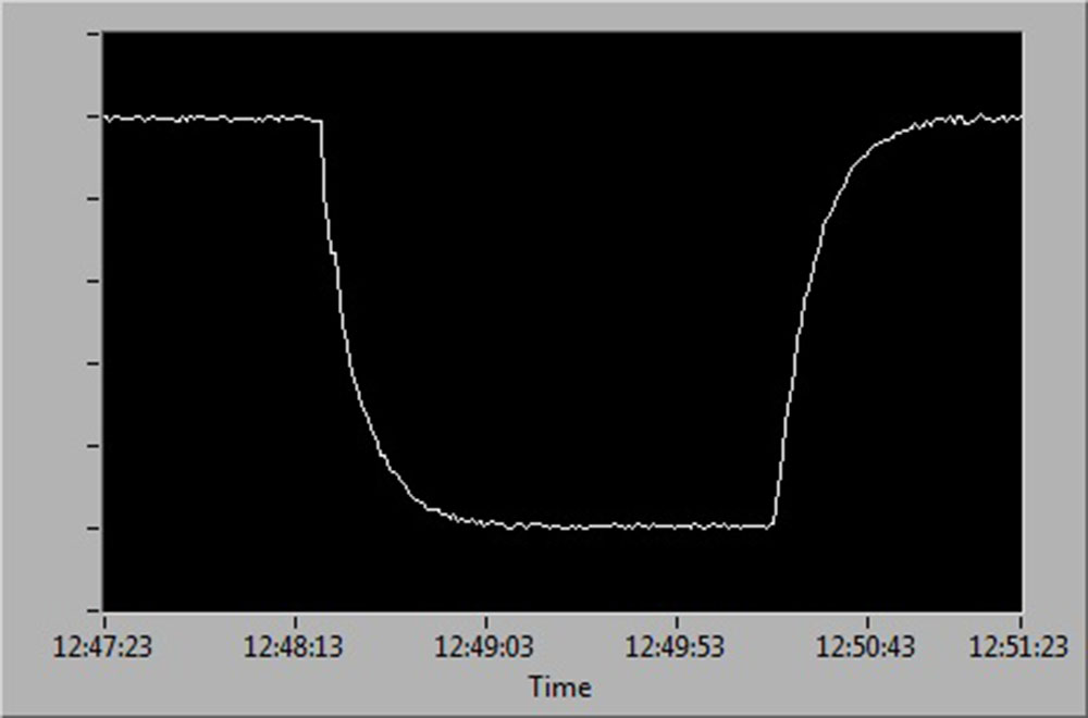 |
|
| 100% to 0% to 100 % air saturation | |
How to mount a sensor spot?
The oxygen sensor spot should be integrated into a dry, clean vessel (humidity or oily residues affect the adhesion and may lead to a detaching of the sensor spot from the vessel wall). The adhesion surface area of the vessel wall should be plane or slightly arched but not strongly curved or corrugated. Otherwise, the spot may detach partly from the vessel wall during the curing process of the silicon glue due to the tension of the spot.
The silicon glue should be cured for at least 60 min. before the test vessel is fill.
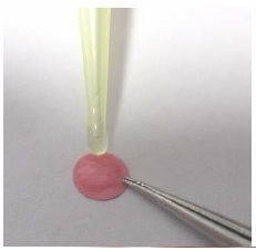
Apply a small amount of silicon glue (D5-Spot: ca. 4 µL) onto the red side of the spot.

Position the spot on the plane bent end of a spatula.
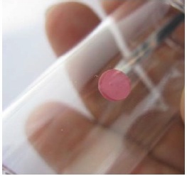

Attach the spot to the inside wall of the test vessel.
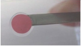
Shift the sensor spot slightly with little pressure onto the surface so that a small ring of silicon glue emerges around its edge.
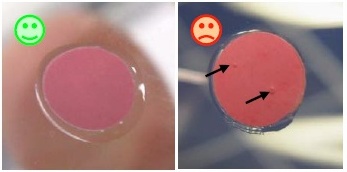
No air should be enclosed in the silicon layer between spot and vessel wall.
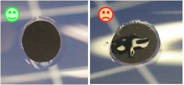
Silicon stains on the black sensor surface should be avoided since they increase the response time of the sensor.
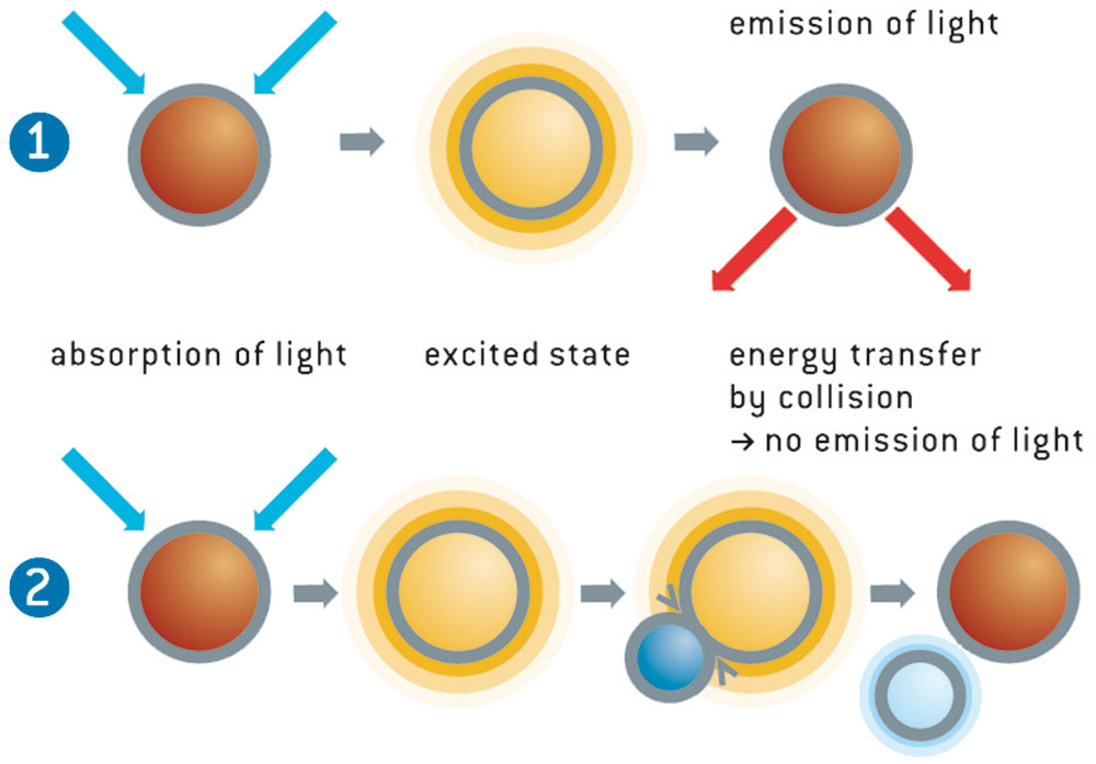
LinkHow do optodes work?
The light from the blue-green LED excites the oxygen sensor to emit fluorescence. If the sensor spot encounters an oxygen molecule, the excess energy is transferred to the oxygen molecule in a non-radiative transfer, decreasing or quenching the fluorescence signal. The degree of quenching correlates to the partial pressure of oxygen in the matrix, which is in dynamic equilibrium with oxygen in the sample. The decay time measurement is internally referenced.
What is a Shuttle Box?
The Loligo® shuttle tanks are modified versions of the classic operant conditioning chambers (also known as the Skinner box) used for experimental analysis of behavior, e.g. to study operant conditioning and classical conditioning in animals.
An operant conditioning chamber permits experimenters to study behavior conditioning (training) by teaching a subject animal to perform certain actions (like pressing a lever) in response to specific stimuli like a light or sound signal. When the subject correctly performs the behavior, a mechanism delivers food or another reward. In some cases, the mechanism delivers a punishment for incorrect or missing responses.
With this apparatus, experimenters perform studies in conditioning and training through reward/punishment mechanisms. Operant chambers have at least one operandum, that can automatically detect the occurrence of a behavioral response or action.
Typical operanda for primates and rats are response levers. Despite such a simple configuration (e.g. one operandum and one feeder), it is possible to investigate many psychological phenomena in this way.
For this reason, operant conditioning chambers have become common in a variety of research disciplines including behavioral pharmacology, and Skinner's Box have been used extensively for behavioral research in primates and rats.
Loligo® shuttle tanks have been developed for aquatic animals, like zebrafish or crustaceans, and the tank design allows for independent control of water quality in two sub compartments. Tank dimensions are made special to accomodate a wide variaty of animal species and sizes.
Inside the Shuttle tank, the animal can freely "shuttle" between two sub compartments with opposite acting controls.
The computerized Loligo® shuttle systems are equiped with a video camera and lighting conditions enabling real-time pc vision software to detect animal locomotion.
If the animal changes its position from one user-defined zone to the next through locomotion, the computer software (ShuttleSoft) activates/deactivates programmed devices to change environmental conditions inside the tank, e.g. to regulate water temperature to preferred values through behavior. Or you can set up two different (constant) temperature levels in the two tank compartments independent of fish behavior for exposure/avoidance/choice tests.
Today, a main application of Loligo® shuttle tanks measurements of temperature preference in aquatic ectotherms (as well as avoidance behavior), and automated computerized systems, have been made for a range of other environmental factors like water turbidity, salinity, oxygen saturation, pH and pCO2.
The turnkey systems offered include everything needed for video behavior analysis as well as monitoring and regulating water quality.
LinkWhat is intermittent respirometry?
The following references offer a good start to understanding the principles, methods, and what to look out for when studying intermittent respirometry in aquatic organisms:
- A large aerobic scope and complex regulatory abilities confer hypoxia tolerance in larval toadfish, Opsanus beta, across a wide thermal range
LeeAnn Frank, Joseph Serafy, Martin Grosell (2023)
Science of the Total Environment
Link to article - Methods for Fish Biology, 2nd edition
Timothy D. Clark (2022)
Respirometry. Pages 247–274 in S. Midway, C. Hasler, and P. Chakrabarty, editors. Methods for fish biology, 2nd edition. American Fisheries Society, Bethesda, Maryland.
Link to article - Guidelines for reporting methods to estimate metabolic rates by aquatic intermittent-flow respirometry
Shaun S. Killen, Emil A. F. Christensen, Daphne Cortese, Libor Závorka, Tommy Norin, Lucy Cotgrove, Amélie Crespel, Amelia Munson, Julie J. H. Nati, Magdalene Papatheodoulou, David J. McKenzie (2021)
Journal of Experimental Biology
Link to article - Effects of social and visual contact on the oxygen consumption of juvenile sea bass measured by computerized intermittent respirometry
J. Herskin (2005)
Journal of Fish Biology
Link to article - Some errors in respirometry of aquatic breathers: How to avoid and correct for them
J. F. Steffensen (1989)
Fish Physiology and Biochemistry
Link to article
Intermittent flow (or stop-flow) respirometry - Principles and Background
Measurements of oxygen consumption rates on fish and other water breathers commonly involves using one of three different methods:
1. Closed respirometry (or constant volume respirometry)
2. Flow-through respirometry (or open respirometry)
3. Intermittent flow respirometry (or stop-flow)
1. Closed respirometry (or constant volume respirometry)
Measurements in a sealed chamber of known volume (a closed respirometer). The oxygen content of the water is measured initially (t0), then the respirometer is closed and at the end of the experiment (t1) the oxygen content is measured again.
Knowing the body weight of the animal, the respirometer volume and the oxygen content of the water at time t0 and t1, the mass specific oxygen consumption rate (mg O2/kg/hour) can be calculated as follows:
VO2 = ([O2]t0 – [O2]t1) • V/t/BW
- [O2]t0 = oxygen concentration at time t0 (mg O2/liter)
- [O2]t1 = oxygen concentration at time t1 (mg O2/liter)
- V = respirometer volume minus volume of experimental animal (liter)
- t = t1 – t0 (hour)
- BW = body weight of experimental animal (kg)
An advantage of this method is its simplicity. A disadvantage is that the measurements are never made at a constant oxygen level, due to the continuous use of oxygen by the animal inside the respirometer. This might cause problems when interpreting data, since animal respiration often changes with ambient oxygen partial pressure.
Furthermore, metabolites from the experimental animal, i.e. CO2, accumulate in the water, thus limiting the duration of measurements. This limited time for measurements prevents the experimental animal to recover from initial handling stress that often increase fish respiration significantly and for several hours, thus overestimating oxygen consumption rates.
2. Flow-through respirometry (or open respirometry)
This is a more sophisticated method for oxygen consumption measurements. Experimental animals are placed in a flow-through chamber with known flow rate. Oxygen is measured in the inflow and outflow and oxygen consumption rate (mg O2/kg/hour) can be calculated as:
VO2 = F • ([O2]in – [O2]out)/BW
- F = water flow rate (l/hour)
- [O2]in = oxygen content in water inflow (mg O2/liter)
- [O2]out = oxygen content in water outflow (mg O2/liter)
- BW = body weight of experimental animal (kg)
The advantages of this method are several:
- The duration of the experiment is in principle unlimited
- No accumulation of CO2 and other metabolites
- Its possible to measure at a constant oxygen level
- By controlling the quality of the inflowing water its possible to measure metabolism at different desired levels of oxygen, salinity etc.
However, this method bring along one significant disadvantage: In order to determine oxygen consumption by open respirometry it is crucial that the system is in steady state. This means that the oxygen content of the in-flowing and out-flowing water, AND the oxygen consumption of the animal, have to be constant.
If the oxygen consumption of the animal for some reason changes during the experiment, steady state will not exist for a while. The above formula will not give the correct oxygen consumption rate until the system is in steady state again. The duration of the time lag depends on the relationship between chamber volume and flow rate. Thus, open respirometry measurements have poor time resolution and are not suitable for determination of oxygen consumption on organisms with a highly variable respiration like fish.
3. Intermittent flow respirometry
Our system for automatic respirometry works by intermittent flow respirometry aiming at combining the best of both 1) closed and 2) flow-through respirometry.
- The experimental animal is placed in a respirometer immersed in an ambient tank (temperature bath).
- A recirculating pump ensures proper mixing of the water inside the respirometer and adequate flow past the oxygen probe.
- A second pump can swap the water inside the respirometer with water from the ambient tank (temperature bath). During measurements of oxygen consumption, this flush pump is turned off and the systems operates like a closed respirometry setup.
- Then the pc controlled flush pump turns on pumping ambient water into the respirometer and bringing the oxygen content back to pre measurement levels.
In this way, problems with accumulating metabolites and severe changes in oxygen level due to animal respiration are avoided. - As with open respirometry, the duration of the experiment is in principle unlimited.
However, the most important advantage is the great time resolution of this method. Oxygen consumption rates of animals can be determined for every 10th minutes over periods of hours or days, making our systems for automatic respirometry extremely suited for uncovering short term variations (minutes) in respiration.
In summary, our system for automatic respirometry is developed for prolonged and automatic measurements of oxygen consumption rate in a controlled laboratory environment.
The automatic measuring proceedure runs in 3 phases:
- Measuring period
- Flush period
- Wait period
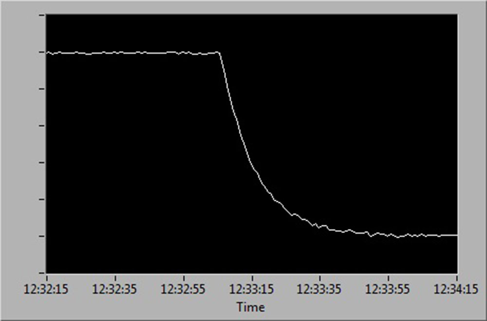
In the Measuring period (1) the flush pump is off, and the chamber is closed. Fish respiration rate is calculated from the decline in oxygen. During this time the recirculation pump is active to mix the water inside the respirometer and to ensure proper flow past the oxygen sensor.
The measuring period is followed by a Flush period (2) where the flush pump is active pumping water from the ambient temperature bath and into the respirometer. During this period the recirculation pump is inactive and the oxygen curve will raise to approach the level of the amient water.
Finally, the flush pump stops and the loop ends with a short Wait period (3) before starting a new measuring period. This waiting period is necessary to account for a lag in the system response resulting in a non-linear oxygen curve. During the Wait period the recirculation pump is active.
Examples of raw MO2 data
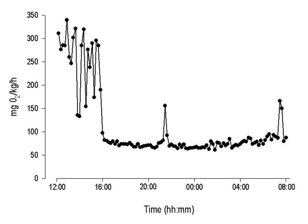
Standard metabolic rate of juvenile Rainbow Trout was determined in static respirometer chambers and with an automated respirometry system from Loligo® Systems. Initial high oxygen consumption rates due to handling stress, were followed by a gradual decline to lower and more stable values indicating standard metabolic rate for the specimen. Notice the high temporal resolution (10 min) of the system revealing sudden changes in MO2.
Courtesy by J.Svendsen/DIFRES & J.Lund/Univ. Aarhus
LinkWhat chamber sizes will fit my animal?
The chamber should be large enough to house the intact animal, but not much larger as it will leave space for unwanted activity like swimming that will make it harder (and take longer) to determine resting/standard/minimum metabolic rate.
The chamber volume should be kept at a minimum for reliable respiration measurements to get a better temporal resolution and signal-to-noise ratio. If the volume is too large, the resulting oxygen depletion curve will be too flat for solid estimates of the slope that is used in the calculation of the oxygen consumption rate (MO2).
As a rule of thumb, we recommend a resting chamber with a volume 10-50 times the volume (≈ wet weight) of the animal:
Use a 50 mL chamber for fish weighing down to 1 g (ratio = 50/1 = 50).
A lower ratio might be needed as the mass specific respiration rate of ectotherm animals, like fish, scales with body size (i.e., large animals have lower mass specific O2 consumption rates than smaller animals) and temperature (i.e., high temperature = high respiration and vice versa), and also differs between species (e.g., a sluggish benthic fish species often have a lower mass specific metabolic rate than an active pelagic species).
Thus, use a smaller chamber (ratio) if working with large and sluggish arctic fish, e.g., a 10 L chamber for fish weighing down to 1 kg fish (ratio = 10/1 = 10).
LinkWhat swim tunnel should I choose?
Active fish swimming in a tunnel respirometer have high mass-specific oxygen consumption rates (MO2), allowing reliable oxygen consumption estimates in relative higher respirometer volume than for static respirometry. Tunnel respirometers are difficult to build with a fish volume to respirometer volume of less than 1:100. We recommend a maximum ratio between the wet weigth (or volume) of the fish and the volume of the swim respirometer of 1:200, e.g. a 90 liter swim respirometer fits fish down to app. ½ kg. If the volume is too large, the resulting oxygen curve will be too flat for reliable estimates of the slope that is used in the calculation of oxygen consumption rate (MO2).
Another restraint is the dimensions of the test section, which should allow the experimental fish to perform unrestricted swimming. This will largely depend on the species and mode of swimming.
Please contact us to get free advice on which swim tunnel that will be best for your project.
LinkWhat pump flow is needed for my chamber?
To wash out a tube-shaped respirometer chamber requires a volume ~5 times that of the chamber.
Thus, if you use a pump delivering a flow per minute equal to the chamber volume, then a 5 minutes flush period will ensure that 99 % of the water is replaced during each flushing cycle.
Stronger pumps might create too strong a flow forcing fish to struggle or unwanted activity. Lower flows require longer time for flushing, and this will decrease time resolution of MO2 data.
LinkAre glass chambers better than plastic chambers?
Some materials, like Plexiglass/Perspex can act as oxygen stores and sinks, forming pools of oxygen which can be released or stored in a reversible way - see Stevens, J. (1992) J. Appl. Physiol. 72, 801-804.
This can have an important effect when chambers are down-scaled for micro respirometric measurements of very low oxygen fluxes.
Thus, for oxygen measurements in small volumes less than a few millilitres (mL), we recommend chambers of glas and inert components with non or low oxygen storage capacity!
For respirometers with larger volumes (>½ litre), the use of acrylic materials have no significant effects on measurements.
LinkHow to update license information in WIBU dongles?
If you purchased a software upgrade, please follow the steps below to add new license codes to your WIBU dongle:
- Download the following info file (LINK) and save the file to your desktop.
- Double-click it to transfer license codes from your dongle (connected to your PC) and save it to a .wbc file.
- Email the .wbc file to this address: mail@loligosystems.com.
- We will then quickly return a .rtu file as an email attachment. This .rtu file carries the new license code(s).
- Save the .rtu file on your desktop.
- Double-click the .rtu file to transfer new license code(s) to the dongle connected to your PC.
- Finally, download the upgraded version of the software from our website and install it.
Ambient O2: NaN-error
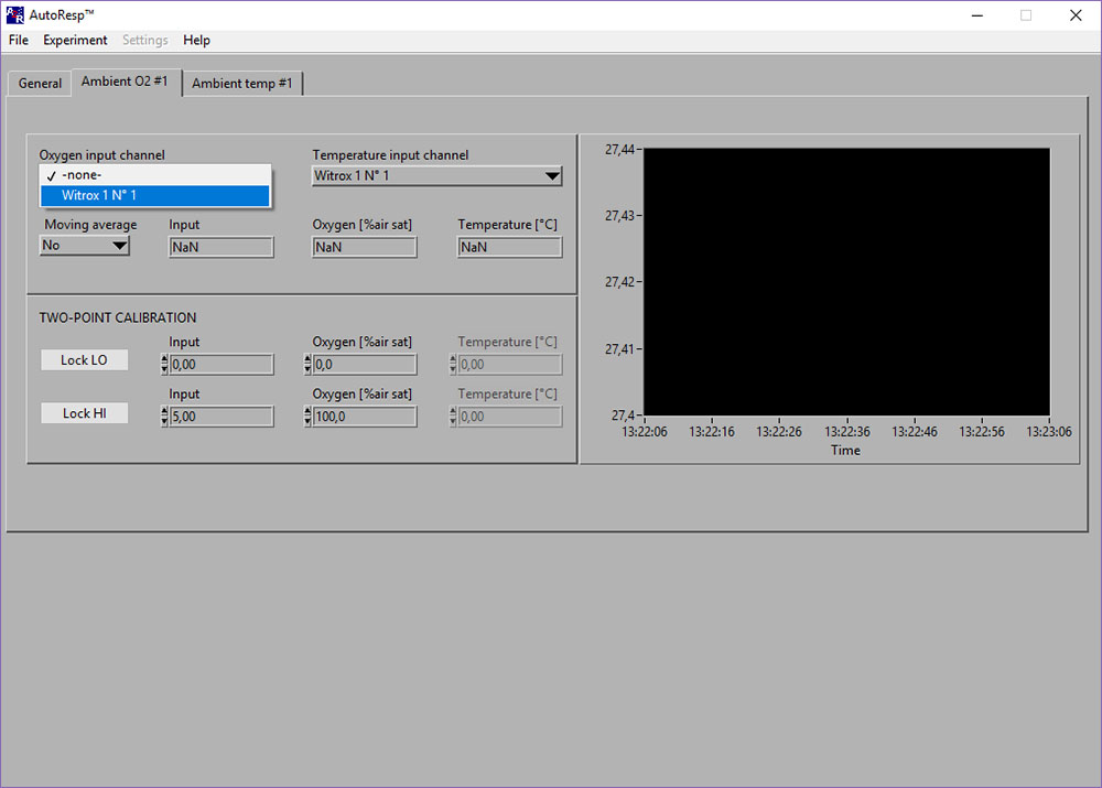
If the Input [phase], Oxygen [%air sat] and Temperature [OC] shows NaN (Not a Number), you should check the following:
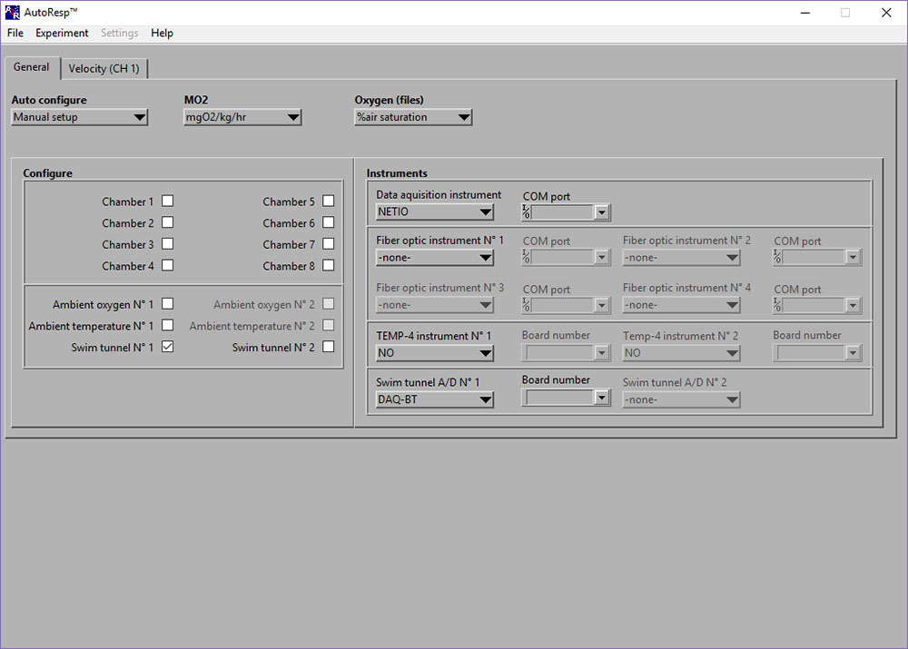
- Select the right Witrox instrument for the Oxygen input channel (see image above)
- Select the right Witrox instrument for the Temperature input channel (for real-time compensation).
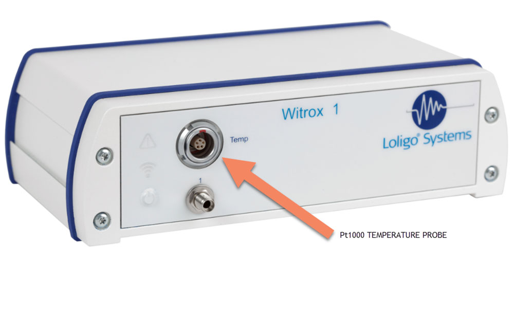
- Check that the fiber optic cable and the Pt1000 temperature probe (red mark on cable must match red mark on Temp input) is connected correctly to the Witrox instrument (see below):
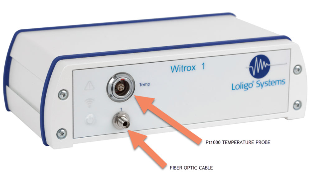
The NaN should now be replaced by data values.
LinkAmbient temp: NaN-error

If the Input [phase] and Temperature [OC] shows NaN (Not a Number), you should check the following:
- Select the right Witrox instrument for the Temperature input channel (see image above).
- Check that the Pt1000 temperature probe is connected correctly (red mark on cable must match red mark on Temp input) to the Witrox instrument:
The NaN should now be replaced by data values.
LinkDAQ-BT board number disappears when I select it in AutoResp?
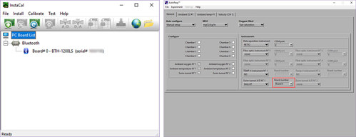
If the Board number for the DAQ-BT disappears after having selected it, there could be two reasons:
- You have not selected the correct board number.
- A board number has not been configured for the device.
Solutions:
- Select the board number that has been configured for the instrument.
- Tip: Open the software InstaCal to check the correct board number (here Board# 0):
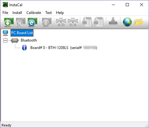
- Tip: Open the software InstaCal to check the correct board number (here Board# 0):
- Configure a board number for the DAQ-BT device.
- Exit AutoResp.
- Open the software InstaCal as administrator (right-click).
- InstaCal will now configure the instrument automatically. Click OK to the following message:
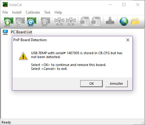
- Click OK to the following message:
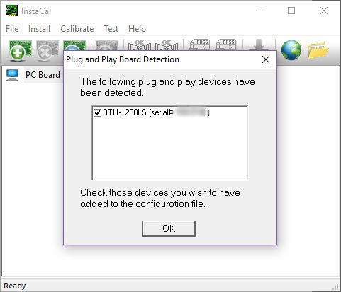
- Use the board number you see here (e.g. Board# 0):
- Click File > Exit
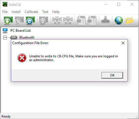
- If the following error message appears, you must exit InstaCal and open it again as administrator:
- Exit AutoResp.
Calibration error: Ambient oxygen No 1
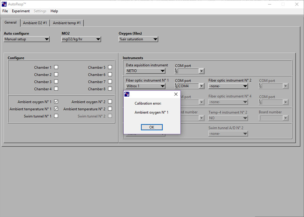
ERROR: Instrument 1 (Please make sure the instrument is in range and turned ON)
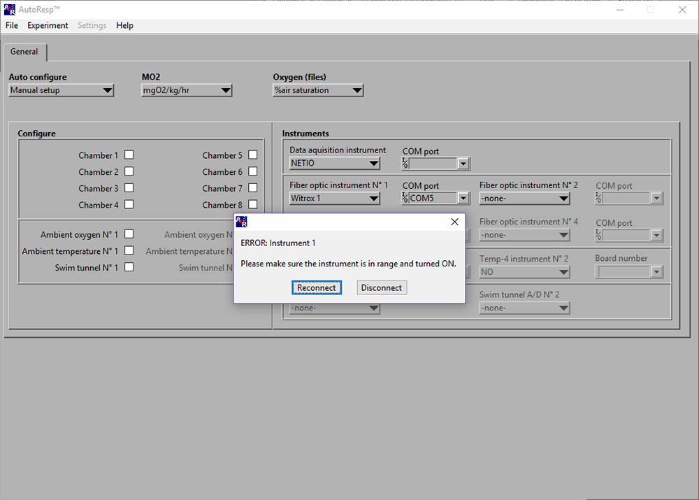
If the ERROR: Instrument 1 (or 2/3/4) appears, you should check:
- If you have selected the assigned COM port for the Witrox instrument.
- If the Witrox instrument is ON and within (Bluetooth) range of the computer.
- If the Witrox instrument is paired with the computer.
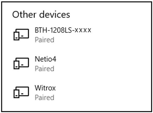
- Tip: Check your connected Bluetooth devices list (see Other devices).
- If the Witrox instrument has timed-out (warning icon on the instrument will light red when timed-out).
Solution:
Close the error-window.
- To find the assigned COM, please try:
- In Windows 10: Go to Control Panel > Devices and Printers > Find the paired Witrox device > Right-click on the device icon > Choose Properties > Choose the Hardware tab > Look for the COM port under Standard Serial Connection via Bluetooth (COM#) > Use this COM-port in AutoResp™.
- Turn the Witrox instrument ON and secure a free line of sight to the computer avoiding metal or magnetic objects that can block wireless communication.
- To pair the Witrox instrument to your computer, please try:
- In Windows 10: Go to Settings > Devices > Add Bluetooth or other device > Choose Bluetooth > Look for Witrox and choose “Pair”. If Windows asks for a pairing code, use “0” (zero).
- Press the power button to turn the Witrox instrument OFF and exit the timed-out mode. Press the power button again to turn the Witrox instrument ON.
No COM port selected for fiber optic instrument No 1
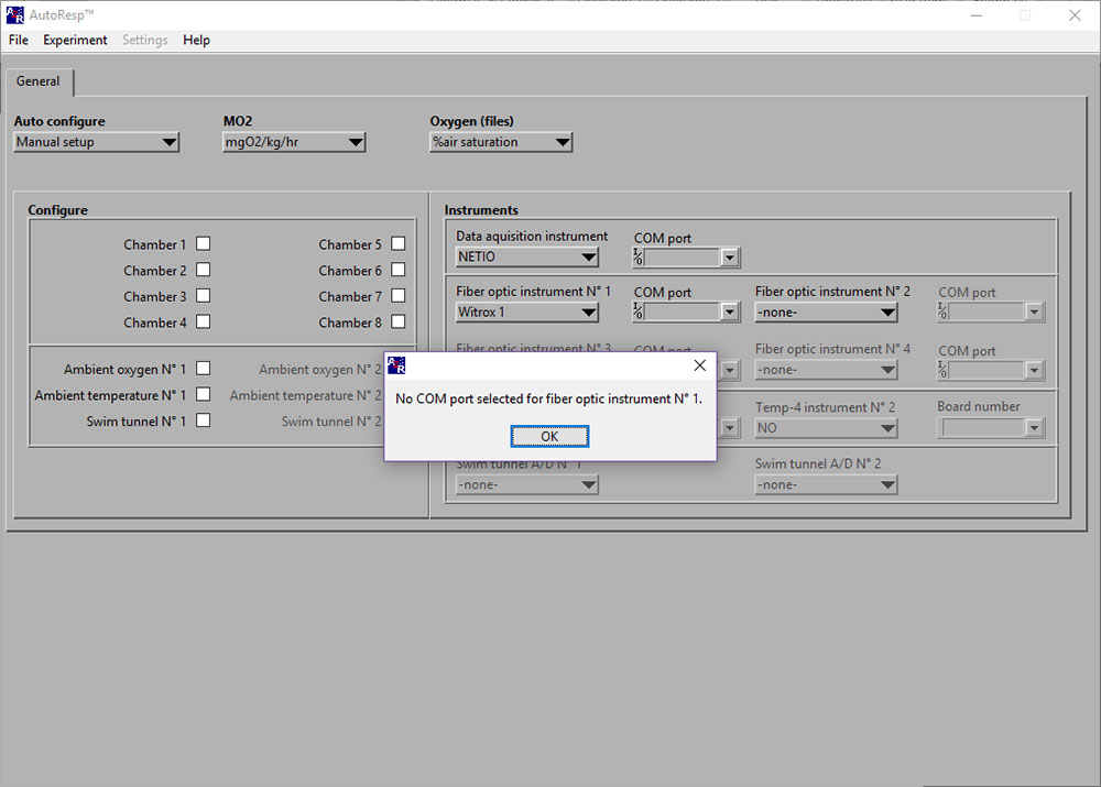
If the No COM port selected error message appears, you should check that you have selected the assigned COM port for the instrument indicated in the error window; here the first oxygen instrument, a Witrox 1.
LinkNo input for: Ambient oxygen No 1

If the No input for: Ambient oxygen No 1 error message appears, you should check:
- If the oxygen sensor (fiber optic cable) is connected correctly to the Witrox instrument SMA connector:
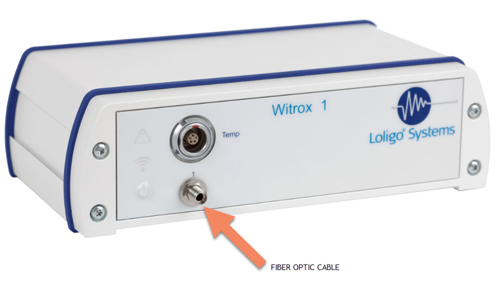
- If the fiber optic cable is damaged.
- If the fiber optic cable is misaligned onto or at a distance from the sensor spot.
No input for: Ambient temperature No 1
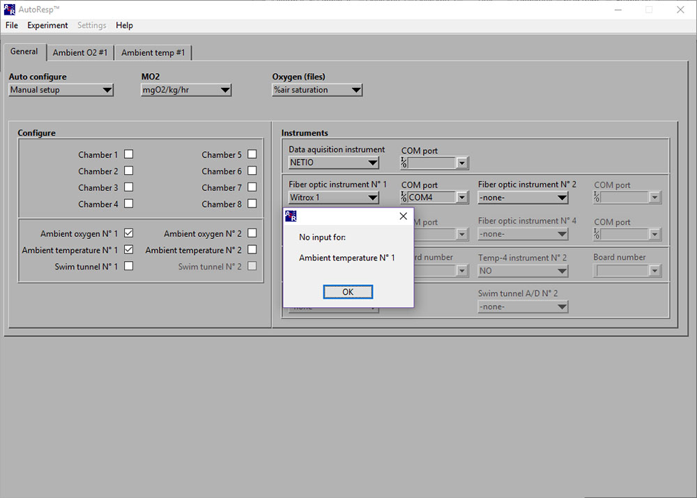
If the No input for: Ambient temperature No 1 error message appears, you should check that the Pt1000 temperature probe is connected correctly to the Witrox instrument (red mark on cable must match red mark on Temp input):
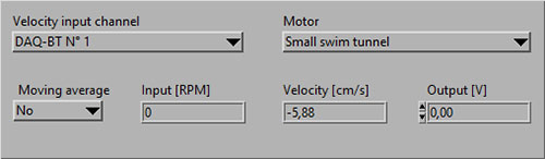
Velocity (CH #): NaN-error
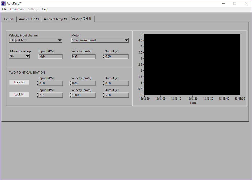
If the Input [RPM], Velocity [cm/s] or Output [V] shows NaN (Not a Number), you should check the following:
- That the motor controller is powered ON and set to FWD/Forward.
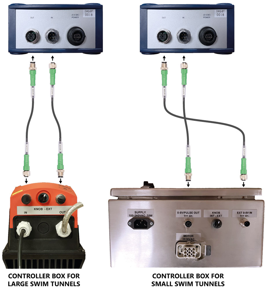
- That the OUT/IN on the back of the DAQ-BT is connected with the analog data cables to the IN/OUT on the motor controller:
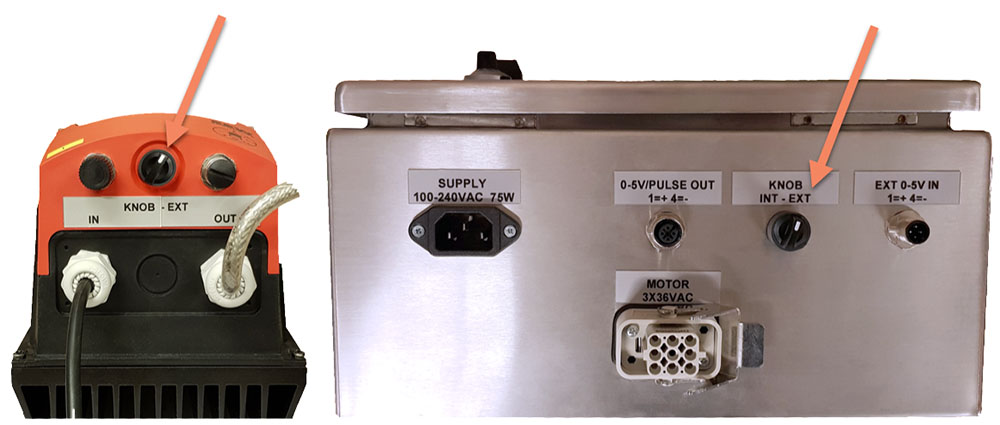
- That the knob on the motor controller is turned towards EXT:
- That you have selected the DAQ-BT for the Velocity input channel and the correct Motor (type of swim tunnel):
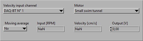
- You should now see data (RPM) values instead of NaN:
No device selected
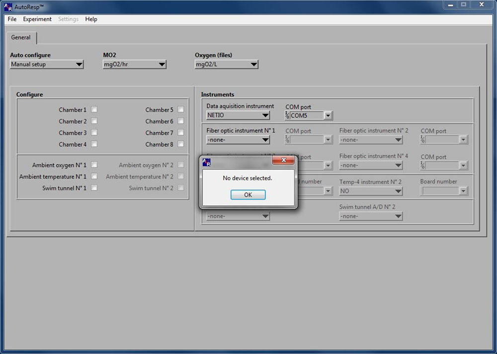
If the No device selected error message appears in AutoResp™ 2.3.0, you should delete the AutoResp configuration file:
NOTE: This will delete all setup settings in AutoResp™.
- Close AutoResp and all applications on your PC.
- In Windows, go to: My computer > Programs (x86) > AutoResp > Delete the CONF-file named AutoResp™.
- Open AutoResp™ as administrator (you should always open as administrator).
- The configuration file has now been reset and the error message should no longer appear.
How do I set up LoligoBT in AutoResp 2.3.0?
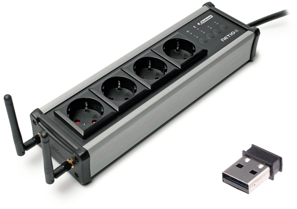
The LoligoBT is a 4-fold power strip that is powered from a wall outlet and communicates with a Windows computer via Bluetooth 4.0. LoligoBT is used for wireless software control of equipment connected to one of the four independent electrical sockets, i.e., relays turning pumps, valves, stirrers etc. ON or OFF from a distance.
Important
- DO NOT reset the LoligoBT device to factory defaults (see How to reset the LoligoBT/Netio device)!
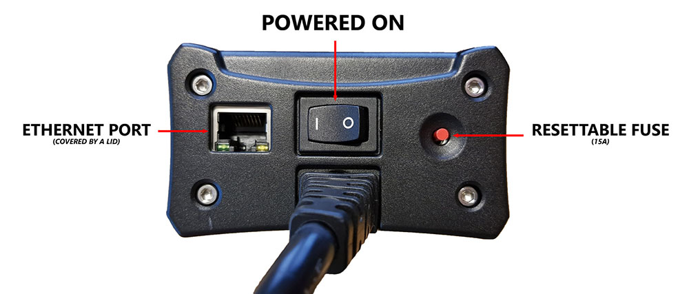
- The LoligoBT is equipped with an ethernet port. The port is covered by a lid. You should NOT remove this lid or connect an ethernet cable to the LoligoBT. It will reset the device and void the warranty!
Setup:
- Insert the small black USB dongle directly into your PC. Let the dongle configure itself in Windows.
- Connect the LoligoBT into a wall socket.
- Set the power switch to “l” to turn the LoligoBT on (see below):
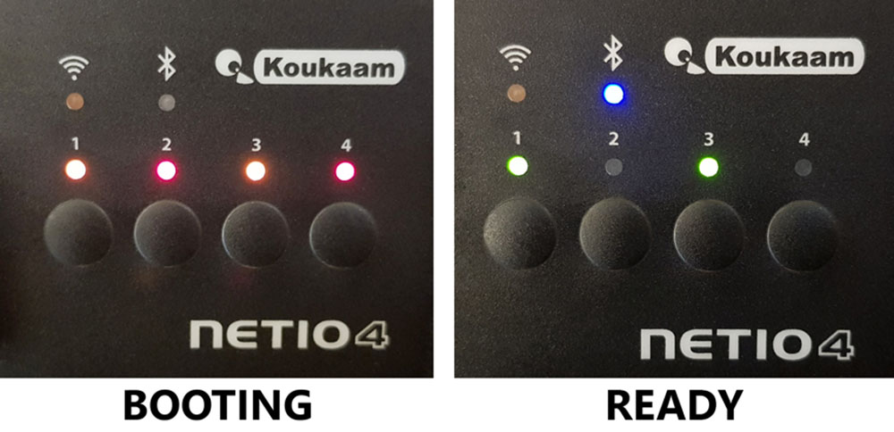
- Wait until the device is ready (see below). It takes about 50 seconds:
- COM port number: In Windows 10, go to Settings > Devices > Look for the BLUEGIGA BLUETOOTH LOW ENERGY (COM#) > Make a note of this COM port number.
- If Windows asks for a pairing code, use “123456”.
- If Windows asks for a pairing code, use “123456”.
- Open AutoResp™ as administrator (right-click).
- Select the right COM port number for this LoligoBT device.
- Your LoligoBT device is now ready to be used in AutoResp™.
How do I set up Witrox 1/Witrox 4 in AutoResp 2.3.0?
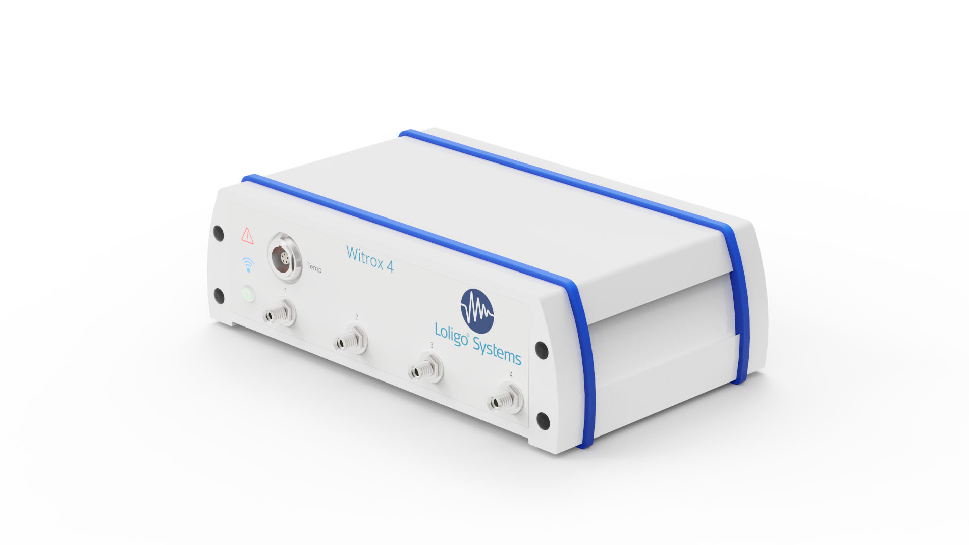
The Witrox instruments are used for measuring dissolved oxygen using fiber optic mini sensors (optodes) and for measuring temperature.
Important
- Do not use the free WitroxView software while running AutoResp™ on the same PC!
Setup
- To power the Witrox instrument, connect the DC adapter to a wall outlet and the USB power cable to the threaded socket on the backside of the instrument.
- Tip: You can power a Witrox instrument directly from your PC using a USB cable.
- Tip: You can power a Witrox instrument directly from your PC using a USB cable.
- Press the power button. The power LED will turn green. The link LED (wireless icon) will flash blue indicating that pairing mode is enabled.
- Pairing in Windows 10: Go to Settings > Devices > Add Bluetooth or other device > Choose Bluetooth > Look for Witrox and choose “Pair”.
- If Windows asks for a pairing code, use “0” (zero).
- If Windows asks for a pairing code, use “0” (zero).
- Verify that the Witrox is paired with your PC (under Devices in Other devices list).
- COM port number: In Windows 10, go to Control Panel > Devices and Printers > Find the paired Witrox device > Right-click on the device icon > Choose Properties > Choose the Hardware tab > Look for the COM port under Standard Serial Connection via Bluetooth (COM#) > Make a note of this COM port number.
- Open AutoResp™ as administrator (right-click).
- Select the right COM port for this Witrox instrument.
- Your Witrox instrument is now ready to be used in AutoResp™.
How do I set up DAQ-BT in AutoResp 2.3.0?
The DAQ-BT device is used for wireless data acquisition from and control of Loligo® swim tunnels. The built-in Bluetooth communication allows you to place the PC at a distance from the swim tunnel. The device has inputs and outputs for controlling and acquiring RPM data from the swim tunnel motor controller (VFC).
Setup
- To power the DAQ-BT device, connect the DC adapter to a wall outlet and the USB power cable to the threaded socket on the backside of the instrument.
- Tip: You can power a DAQ-BT instrument directly from your PC using a USB cable.
- Tip: You can power a DAQ-BT instrument directly from your PC using a USB cable.
- Press and hold the power button until the POWER and STATUS LED flash green. Pairing mode is now enabled.
- Pairing in Windows 10: Go to Settings > Devices > Add Bluetooth or other device > Choose Bluetooth > Look for BTH-1208LS-XXXX and choose “Pair”.
- If Windows asks for a pairing code, use “0000” (four zeros).
- If Windows asks for a pairing code, use “0000” (four zeros).
- Verify that the DAQ-BT is paired with your PC (under Devices in Other devices list):
- Open the program InstaCal (from Measurement Computing) as administrator (right-click).
- InstaCal will now detect and configure the DAQ-BT instrument (see below). Click OK to the following message:

- Click OK to the following message:

- The assigned board number must correspond to the board number used in AutoResp™:
- Click File > Exit
- If the following error message appears, you must exit InstaCal and open it again as administrator:

- Open AutoResp™ as administrator (right-click).
- Select the right board number for this DAQ-BT device.
- Your DAQ-BT device is now ready to be used in AutoResp™.
WARNING: DO NOT reset the device to factory defaults!
Resetting the device to factory defaults will void the warranty and remove the pre-installed Loligo® firmware leaving the device unable to communicate with any Loligo® software.
Ways to reset the device (DON’T!!!)
The LoligoBT/NETIO4All device can be reset to factory defaults in two ways:
- By pressing and holding outlet buttons 1 and 2 when starting the device via power switch. Hold the buttons until the device beeps 3 times. During the resetting process, all the outlet LED are blinking red. As soon as reset is completed, the device beeps 3 times. Whole procedure takes about 2 minutes.
- By removing the protective cap from the ethernet port and connecting the device to a computer with an ethernet cable and resetting the device in your browser.
Contact our technical support if you experience connectivity or performance issue with the LoligoBT/NETIO4ALL.
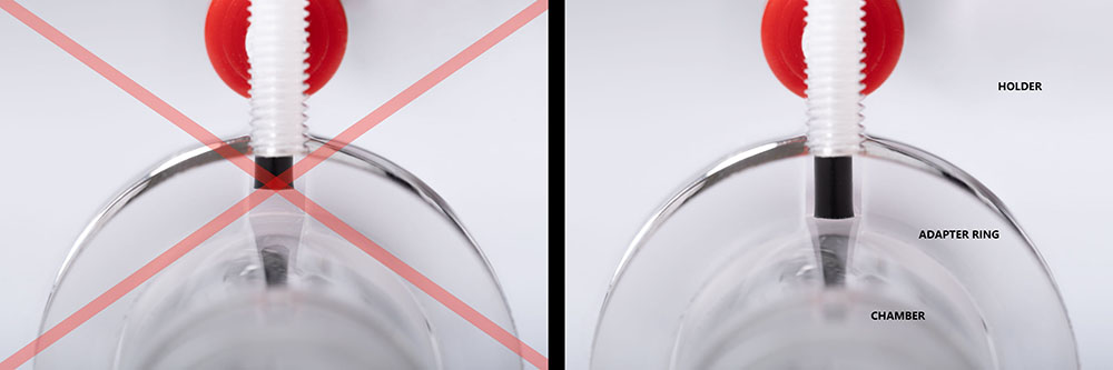
LinkHow to place horizontal mini chambers in holder
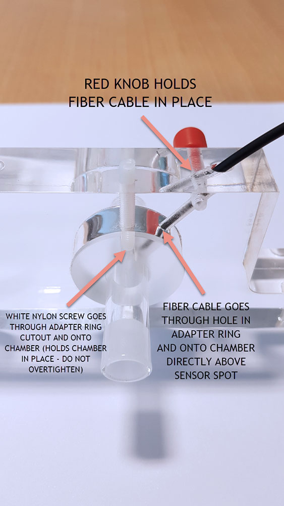
The horizontal mini chambers can be fixed in place in an acrylic holder for easier measurements.
- Place the acrylic adapter ring in the acrylic holder.
- Place the mini chamber (with mounted sensor spot on the inside) inside the adapter ring.
- Rotate the mini chamber so that the sensor spot is located directly below the hole in the adapter ring.
- While keeping the mini chamber in place, tighten the white nylon screw so that it goes through the adapter ring cutout and onto the glass chamber. Tighten until the mini chamber does not rotate/slide. DO NOT OVERTIGHTEN as it will break the mini chamber.
- Push the fiber cable through the angled hole in the holder and place cable tip onto mini chamber, so that it is directly above the sensor spot.
- Tighten red knob to hold fiber cable in place. DO NOT OVERTIGHTEN as it will break the fiber cable.
Copy protection error: No license found
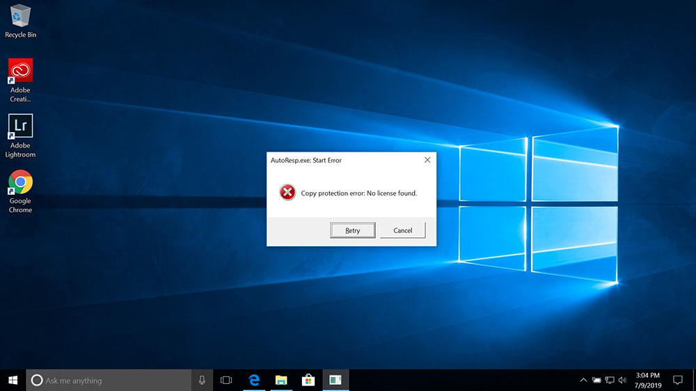
If the Copy protection error message appears when starting a Loligo® software, you should check the following:
- That you have inserted the green WibuKey protection dongle (containing the software license) into your computer:
- That the green WibuKey protection dongle contains the correct software license and not a license for some other Loligo® software.
- If you have installed a newer version of the Loligo® software that you do not have a license for.
- For software upgrades, please follow this FAQ to update your WibuKey dongle license information.
LoliTrack 5 Analysis parameters
Acceleration
- The rate of change of velocity per unit of time.
Acceleration X
- The rate of change of velocity per unit of time along the X-axis.
Acceleration Y
- The rate of change of velocity per unit of time along the Y-axis.
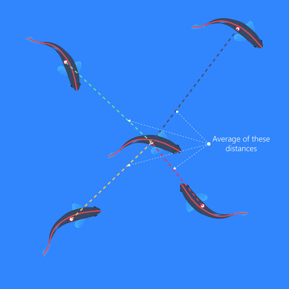
AIID
- (Average Inter-Individual Distance) The average of the distances to all other objects:
Bend
- The angle between a line extending through the center of gravity to the back position, and a line extending through the center of gravity and the front position, e.g., use for tail beat frequency estimation:

Direction of movement
- The direction of movement (in degrees or radians) of the position of the animal. The X and Y direction is defined by the user during the Calibration step:
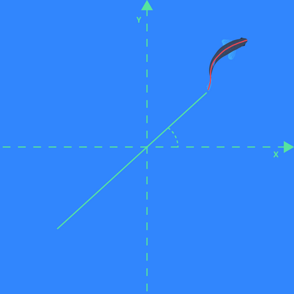
Direction of orientation
- The direction of a line going from the center of gravity position marker to the front position marker of the object:

Distance moved
- Linear displacement of the selected position marker from frame to frame.
Distance to center of zone
- Distance from the selected position marker on the object to the center of the zone(s).
- This parameter is only shown if one or more zones are added in the Analysis tab, and if "Export distance to center of zones" is enabled under Export settings. The parameter data is shown in the sheet for each zone in the Excel file.
Is active?
- Frame to frame object displacement above Activity threshold equals active state (1, in Excel data file) and inactive state (0).
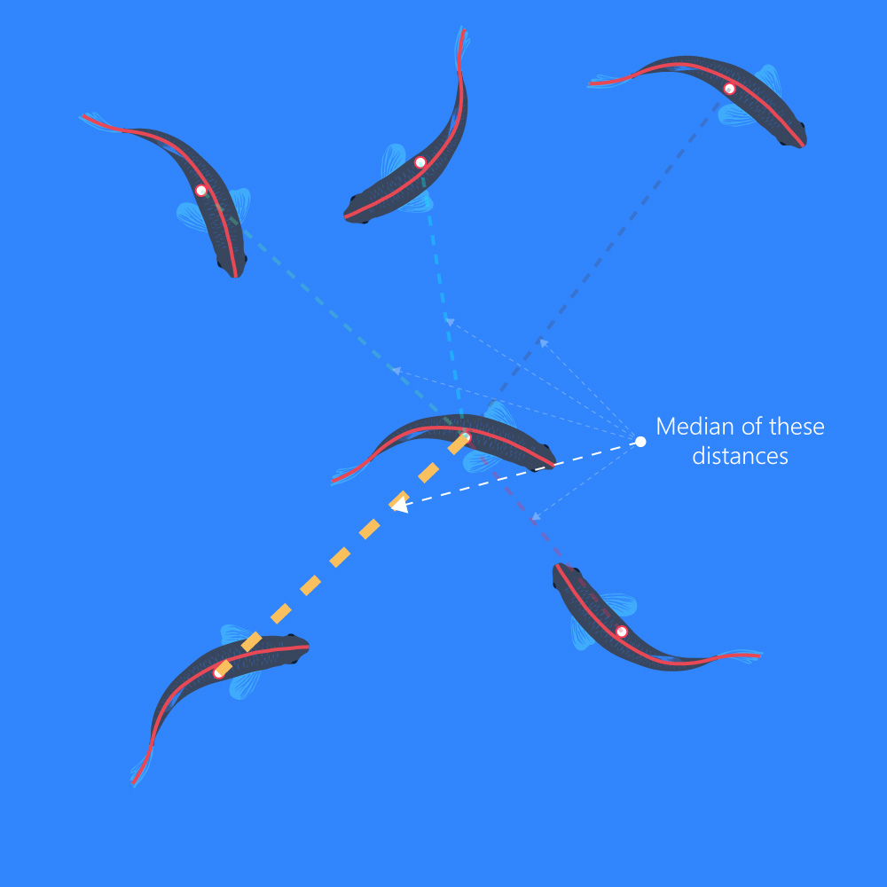
MIID
- (Median Inter-Individual Distance) The median of the distances among all other objects:
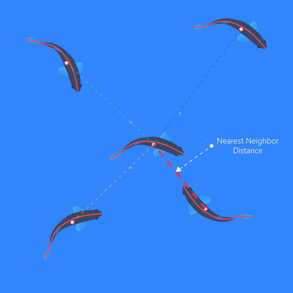
NND
- (Nearest Neighbor Distance) The shortest distance to another tracked object:
Raw X or Y Pos
- The raw pixel values of the positions on the X-axis or Y-axis of the selected position marker of the object. X/Y-origin is in top left corner of the frame:

Calibrated X or Y Pos
- The calibrated positions on the X-axis or Y-axis. X/Y-origin is defined during the Calibration step:

Speed
- Linear displacement of selected position marker per unit of time.
Turning rate movement
- The change in direction of movement per unit of time.
Turning rate orientation
- The change in direction of orientation per unit of time.
Velocity X
- The speed of the object in the direction of the X-axis.
Velocity Y
- The speed of the object in the direction of the Y-axis.
Optimizing your PC for data recording
This guide will help optimizing your PC for data recording. Note that the optimal settings may vary depending on your PC specifications, and that this guide is based on a modern Windows 10 PC.
Dedicate your PC to data recording
Recording data (e.g., video recording) can be a heavy task for many PCs. Therefore, you should make sure that your computer is focusing most of its processing power on this task. Here are some tips on how to do that:
- Close all unnecessary software. Ideally, you should only be running your data recording software (and essential Windows processes), so do not listen to music on YouTube or chat in Microsoft Teams while recording data.
- Prevent process startup. Many processes will start up automatically in the background when you power on your PC. But you can prevent unnecessary processes from doing just that:
- Open the Task manager.
- Open Startup.
- Right-click on the software (that you do not want to start up automatically)
- Choose Disable from the pop-up menu.
- Restart your PC.
- Open the Task manager.
- Go offline. Going offline will prevent many applications from running (also accidentally) during a recording:
- A quick way to go offline is to enable Airplane mode.
- Click on the internet icon in the tool bar.
- Enable Airplane mode.

- A quick way to go offline is to enable Airplane mode.
- Pause Windows updates. You can pause Windows updates to avoid disruptions during recording. Here is how:
- Click on the Windows icon
 .
. - Open the Settings menu
 .
. - Go to Update & Security.
- Go to Windows Update.
- Choose the option Pause updates for 7 days.
- If you want to resume the updates before the 7 days have passed, click the Resume updates button near the top.
- Click on the Windows icon
- Turn off antivirus. Turning off your antivirus software can free up processing power. Remember to turn it back on again after recording.
- Choose correct USB port. If you are using USB devices (like one of our uEye cameras), you must connect the camera to an optimal USB port on the computer: USB 3 devices should be connected to a USB 3 port.
- Enable "Performance mode". Many laptops uses "best battery mode" when running on their battery only which results in reduced performance. Enable "best performance mode" instead and make sure the laptop is plugged in.
- Fingers off your PC! Once your data recording has started, you should not operate your PC – even moving the mouse curser can lower your PC’s performance!
Application requires WibuKey Runtime Modules with version 5.20 or higher
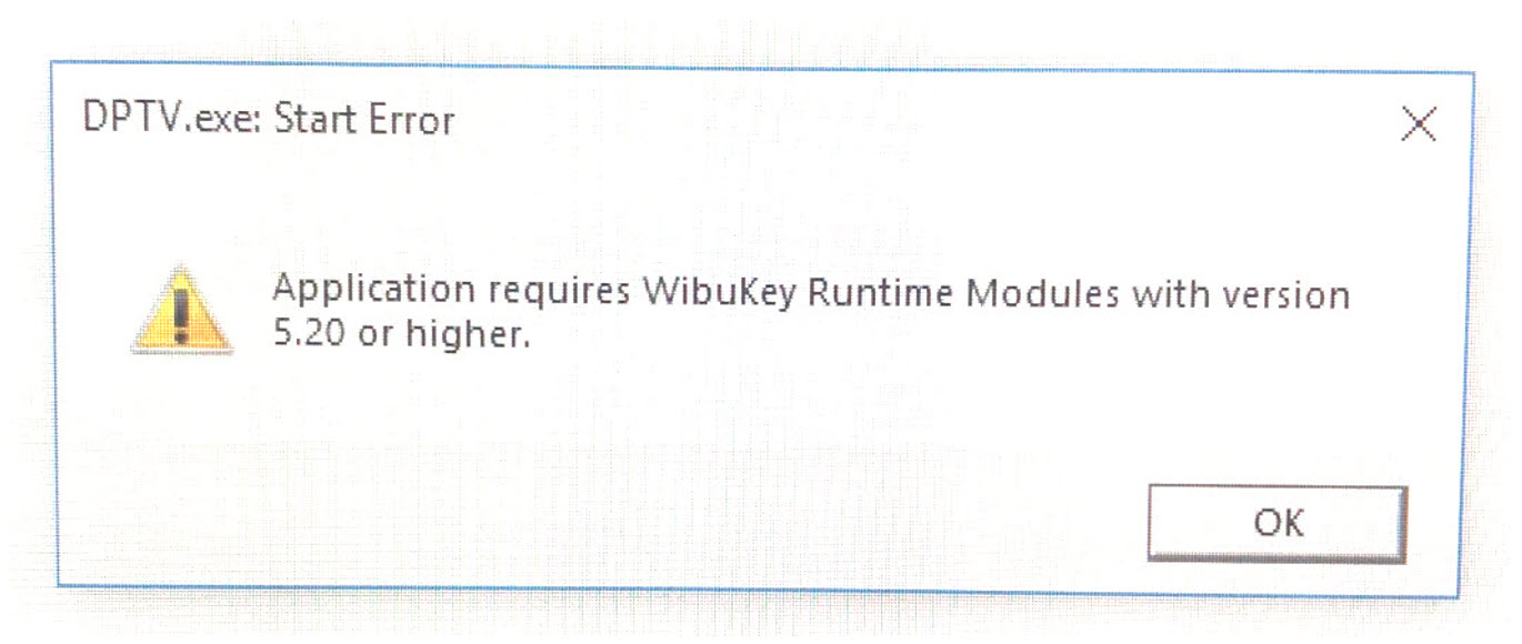
If the “Application requires WibuKey Runtime Modules with version 5.20 or higher” error occurs, here is what to do:
- Unplug the green WibuKey dongle from your computer
- Uninstall the Loligo® software, that gives you the error, from your computer (using Remove App in Windows 10)
- Uninstall WibuKey Setup (WibuKey Remove) from your computer (using Remove App in Windows 10)
- Restart your computer
- Download the version of the Loligo® software, that gave you the error, from our website:
Loligo® Systems. Software Downloads (loligosystems.com) - Install the Loligo® software + WibuKey part as administrator on your computer
- Restart your computer
- Insert green WibuKey dongle into an available USB port on your computer
- Open the Loligo® software as administrator. The error should no longer appear.
ShuttleSoft 3 analysis parameters
This is an in-depth description of each data parameter in the Data Analysis menu in ShuttleSoft 3. Please also see step 26 in the Quick guide for ShuttleSoft 3.
Distance moved (high zone)
- The distance of a single object’s movement in the high zone.
Distance moved (low zone)
- The distance of a single object’s movement in the low zone.
Distance moved (OFF zone)
- The distance of a single object’s movement in the OFF zone.
Max ox in high zone
- The maximum oxygen level measured in the high zone.
Max ox in low zone
- The maximum oxygen measured in the low zone.
Max temp in high zone
- The maximum temperature measured in the high zone.
Max temp in low zone
- The maximum temperature measured in the low zone since.
Min ox in high zone
- The minimum oxygen level measured in the high zone since.
Min ox in low zone
- The minimum oxygen level measured in the low zone since.
Min temp in high zone
- The minimum temperature measured in the high zone.
Min temp in low zone
- The minimum temperature measured in the low zone.
Number of passages
- The number of passages between zone 1 and 2. This number is incremented when the object moves from one zone to the other.
Oxygen avoidance high
- The average of the oxygen level in the high zone when the object leaves the zone.
Oxygen avoidance low
- The average of the oxygen level in the low zone when the object leaves the zone.
Oxygen avoidance mean
- The average of the Oxygen avoidance low and Oxygen avoidance high.
Preference custom value 1
- The weighted average of the custom value 1 based on the time spent in each zone during the last period specified in the Pref. time MovAvg field in the Data settings menu.
Preference custom value 2
- The weighted average of the custom value 2 based on the time spent in each zone during the last period specified in the Pref. time MovAvg field in the Data settings menu.
Preference oxygen
- The weighted average of the preferred oxygen level based on the time spent in each zone during the last period specified in the Pref. time MovAvg field in the Data settings menu.
Preference temperature
- The weighted average of the preferred temperature based on the time spent in each zone during the last period specified in the Pref. time MovAvg field in the Data settings menu.
Preference temperature (Core)
- The calculated object core temperature based on the Decay value field in the Data settings menu.
Speed
- The average distance moved between frames divided by frame rate, i.e., to get speed data in m, cm, or mm per second.
Temperature avoidance high
- The average of the temperatures in the high zone when the object leaves the zone.
Temperature avoidance high (Core)
- The average of the core temperatures in the high zone when the object leaves the zone.
Temperature avoidance low
- The average of the temperatures in the low zone when the object leaves the zone.
Temperature avoidance low (Core)
- The average of the core temperatures in the low zone when the object leaves the zone.
Temperature avoidance mean
- The average of the Temperature avoidance low and Temperature avoidance high.
Temperature avoidance mean (Core)
- The average of the Temperature avoidance low (Core) and Temperature avoidance high (Core).
Time [%] (OFF zone)
- Time spent in the OFF zone measured in percent.
Time [%] (zone 1)
- Time spent in zone 1 measured in percent.
Time [%] (zone 2)
- Time spent in zone 2 measured in percent.
Time [s] (OFF zone)
- Time spent in the OFF zone measured in seconds.
Time [s] (zone 1)
- Time spent in zone 1 measured in seconds.
Time [s] (zone 2)
- Time spent in zone 2 measured in seconds.
Total distance moved
- The total distance of a single object’s movement. This distance is the sum of Distance moved (low zone), Distance moved (high zone) and Distance moved (OFF zone).
Zone high time [%]
- Time spent in high zone measured in seconds.
Zone high time [s]
- Time spent in high zone measured in seconds.
Zone low time [%]
- Time spent in low zone measured in seconds.
Zone low time [s]
- Time spent in low zone measured in seconds.
ShuttleSoft 3 .csv log file parameters
This is an in-depth description of each data parameter in the .csv data file generated in ShuttleSoft 3, and of the Regulating tab mentioned in step 14 in the Quick guide for ShuttleSoft 3.
Avoidance, high oxygen
- The average of the oxygen levels in the high zone when the object leaves the zone since start of logging.
Avoidance, high temperature
- The average of the temperatures in the high zone when the object leaves the zone since start of logging.
Avoidance, high temperature (Core)
- The average of the object core temperatures in the high zone when the object leaves the zone since start of logging.
Avoidance, low oxygen
- The average of the oxygen levels in the low zone when the object leaves the zone since start of logging.
Avoidance, low temperature
- The average of the temperatures in the low zone when the object leaves the zone since start of logging.
Avoidance, low temperature (Core)
- The average of the object core temperatures in the low zone when the object leaves the zone since start of logging.
Core temperature
- The calculated object core temperature based on the Decay value field in the Data settings menu since start of logging.
Custom unit 1 zone 1
- The value of custom unit 1 in zone 1.
Custom unit 1 zone 2
- The value of custom unit 1 in zone 2.
Custom unit 2 zone 1
- The value of custom unit 2 in zone 1.
Custom unit 2 zone 2
- The value of custom unit 2 in zone 2.
Data point in log
- A continuously increasing data point counter.
Distance moved high zone [length units]
- The distance of a single object’s movement in length units in the high zone since start of logging.
Distance moved high zone [pixels]
- The distance of a single object’s movement in pixels in the high zone since start of logging.
Distance moved low zone [length units]
- The distance of a single object’s movement in length units in the low zone since start of logging.
Distance moved low zone [pixels]
- The distance of a single object’s movement in pixels in the low zone since start of logging.
Distance moved OFF zone [length units]
- The distance of a single object’s movement in length units in the OFF zone since start of logging.
Distance moved OFF zone [pixels]
- The distance of a single object’s movement in pixels in the OFF zone since start of logging.
Elapsed time during log
- The elapsed time since start of logging.
Is assigned oxygen
- Shows whether the oxygen hardware has been assigned to the experiment.
Is assigned temperature
- Shows whether the temperature hardware has been assigned to the experiment.
Is logging
- Shows if data is being logged.
Is recording
- Shows if video is being recorded.
Is regulating dynamic oxygen
- Shows if the experiment is regulating the oxygen level in a dynamic manner.
Is regulating dynamic temperature
- Shows if the experiment is regulating the temperature in a dynamic manner.
Is regulating static oxygen
- Shows if the experiment is regulating the oxygen in a static manner.
Is regulating static temperature
- Shows if the experiment is regulating the temperature in a static manner.
Last located position time stamp
- The last time stamp when one object is found.
Logging parameters are reset now
- Describes if the logging parameters has been reset. If True, all data has been reset.
Max ramping speed, oxygen
- The maximum allowed ramping speed of oxygen level in a dynamic experiment.
Max ramping speed, temperature
- The maximum allowed ramping speed of temperature in a dynamic experiment.
Maximum oxygen
- The maximum allowed oxygen level in a dynamic experiment.
Maximum temperature
- The maximum allowed temperature in a dynamic experiment.
Minimum oxygen
- The minimum allowed oxygen level in a dynamic experiment.
Minimum temperature
- The minimum allowed temperature in a dynamic experiment.
Number of found objects
- The total number of found objects in each frame.
Number of found objects in OFF zone
- The number of found objects in the OFF zone in each frame.
Number of found objects in zone high
- The number of found objects in the high zone in each frame.
Number of found objects in zone low
- The number of found objects in the low zone in each frame.
Number of passages
- Increments each time a zone switch occurs since start of logging.
Oxygen delta
- The oxygen delta value. This is the oxygen level difference that the system tries to maintain between high and low zone.
Oxygen hysteresis
- The oxygen level hysteresis value. If the oxygen level is further from the target value than the hysteresis value, the experiment will actively start regulating to reach the target value at which the regulation will stop.
Oxygen units
- Describes the oxygen unit used in the experiment.
Oxygen zone high
- The measured oxygen level in the high zone.
Oxygen zone low
- The measured oxygen level in the low zone.
Preference custom value 1
- The weighted average of the preferred custom value 1 based on the time spent in each zone during the last period specified in the Pref. time MovAvg field in the Data settings menu.
Preference custom value 2
- The weighted average of the preferred custom value 2 based on the time spent in each zone during the last period specified in the Pref. time MovAvg field in the Data settings menu.
Preference oxygen
- The weighted average of the preferred oxygen level based on the time spent in each zone during the last period specified in the Pref. time MovAvg field in the Data settings menu.
Preference temperature
- The weighted average of the preferred temperature based on the time spent in each zone during the last period specified in the Pref. time MovAvg field in the Data settings menu.
Preference temperature Core
- The weighted average of the calculated object core temperature (which is based on the Decay value field in the Data settings menu) based on the time spent in each zone during the last period specified in the Pref. time MovAvg field in the Data settings menu.
Pressure in hPa
- The atmospheric pressure measured in hPa. This number is used in the oxygen unit conversion.
Salinity in per mille
- The salinity in the tank measured in parts per thousand. This number is used in the oxygen unit conversion.
Speed in length units per second
- The distance moved in the selected length units between frames divided by frame rate.
Speed in pixels per second
- The distance moved in pixels between frames divided by frame rate.
Static oxygen setpoint, zone high
- Describes the target value for the static oxygen level regulation in the high zone.
Static oxygen setpoint, zone low
- Describes the target value for the static oxygen level regulation in the low zone.
Static temperature setpoint, zone high
- Describes the target value for the static temperature regulation in the high zone.
Static temperature setpoint, zone low
- Describes the target value for the static temperature regulation in the low zone.
Temperature delta
- The temperature delta value. This is the temperature difference that the system tries to maintain between high and low zone.
Temperature hysteresis
- The temperature hysteresis value. If the temperature is further from the target value than the hysteresis value, the experiment will actively start regulating to reach the target value at which the regulation will stop.
Temperature zone high
- The measured temperature in the high zone.
Temperature zone low
- The measured temperature in the low zone.
Time spent in high zone
- Time spent in the high zone measured in seconds since start of logging.
Time spent in low zone
- Time spent in the low zone measured in seconds since start of logging.
Time spent in OFF zone
- Time spent in the OFF zone measured in seconds since start of logging.
Time stamp
- The time stamp based on the PC system clock (Live experiment) or the chosen start time for a video file (Video file tracking).
Total distance moved [length units]
- The total distance of a single object’s movement in length units since start of logging. This distance is the sum of Distance moved (low zone), Distance moved (high zone) and Distance moved (OFF zone).
Total distance moved [pixels]
- The total distance of a single object’s movement in pixels since start of logging. This distance is the sum of Distance moved (low zone), Distance moved (high zone) and Distance moved (OFF zone).
Zone 1 is high and zone 2 is low
- Describes if zone 1 is set to high and if zone 2 is set to low. In a dynamic experiment, high zone is equal to the increasing zone, and low zone is equal to the decreasing zone.
Zone high is active
- Describes if the high zone is considered “active” based on the tracking settings. The zone is considered “active” when the objects are deemed found in that zone.
Zone high is regulating oxygen down
- Describes when the oxygen level is being regulated down in the high zone.
Zone high is regulating oxygen up
- Describes when the oxygen level is being regulated up in the high zone.
Zone high is regulating temperature down
- Describes when the temperature is being regulated down in the high zone.
Zone high is regulating temperature up
- Describes when the temperature is being regulated up in the high zone.
Zone low is active
- Describes if the low zone is considered “active” based on the tracking settings. The zone is considered “active” when the objects are deemed found in that zone.
Zone low is regulating oxygen down
- Describes when the oxygen level is being regulated down in the low zone.
Zone low is regulating oxygen up
- Describes when the oxygen level is being regulated up in the low zone.
Zone low is regulating temperature down
- Describes when the temperature is being regulated down in the low zone.
Zone low is regulating temperature up
- Describes when the temperature is being regulated up in the low zone.
Zone switch just occurred
- Describes if the object has moved into a new zone.
How to clean a glass microplate
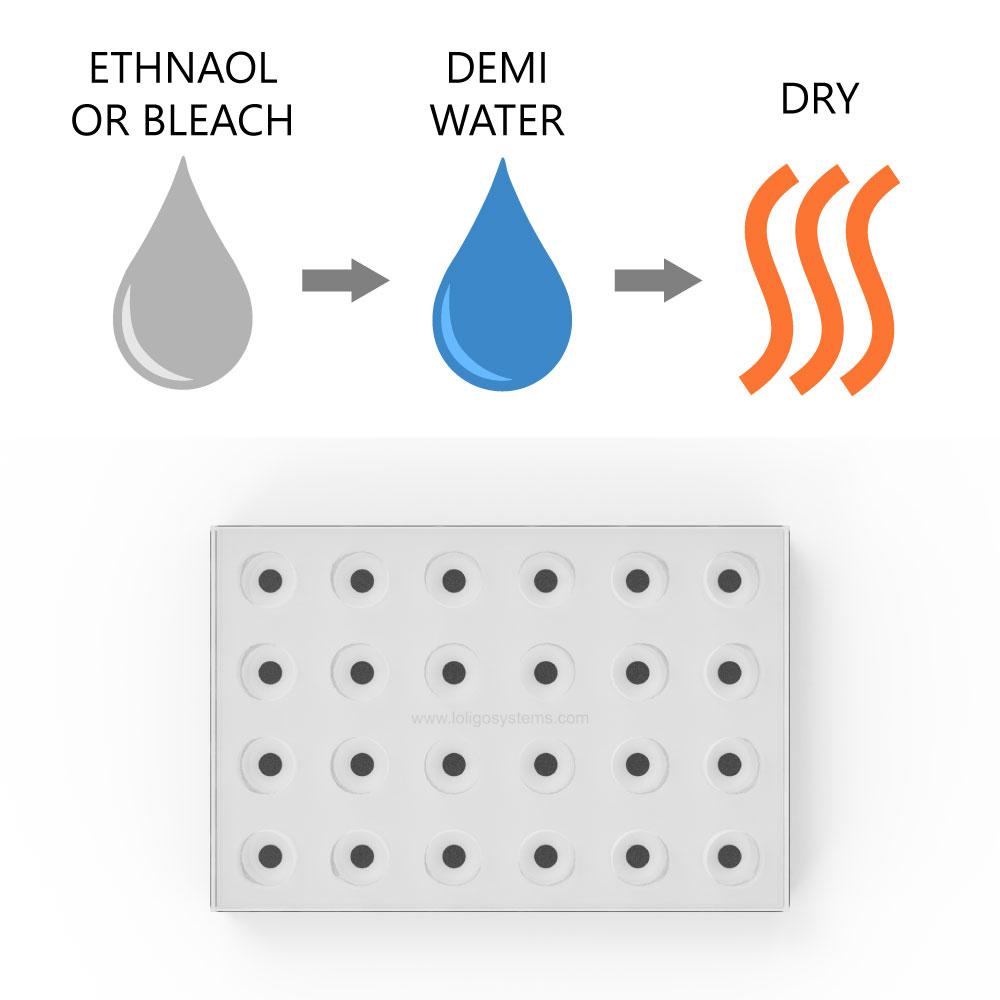
To clean the glass microplate, use ethanol (<70 % v/v), bleach (<3% H₂O₂), or mild detergent, and rinse with demi water. Then dry. If using ethanol to sterilize the spots/wells, then dry the plate thoroughly, at least 2 days at 50-60 °C in an oven, to ensure that all residues have left the sensor dye matrix.
It is recommended to perform a manual calibration after cleaning/sterilizing.
Step-by-Step Instructions using bleach
- Fill each well with 2-2.5% bleach, and ensure that there are no air bubbles in the wells.
- Leave for 10-20 Minutes.
- Empty the wells, and rinse each well thoroughly with demi water.
- Let the wells dry overnight in the dark.
- Perform a manual calibration before starting a new experiment.
Link
How to work with ground glass joints
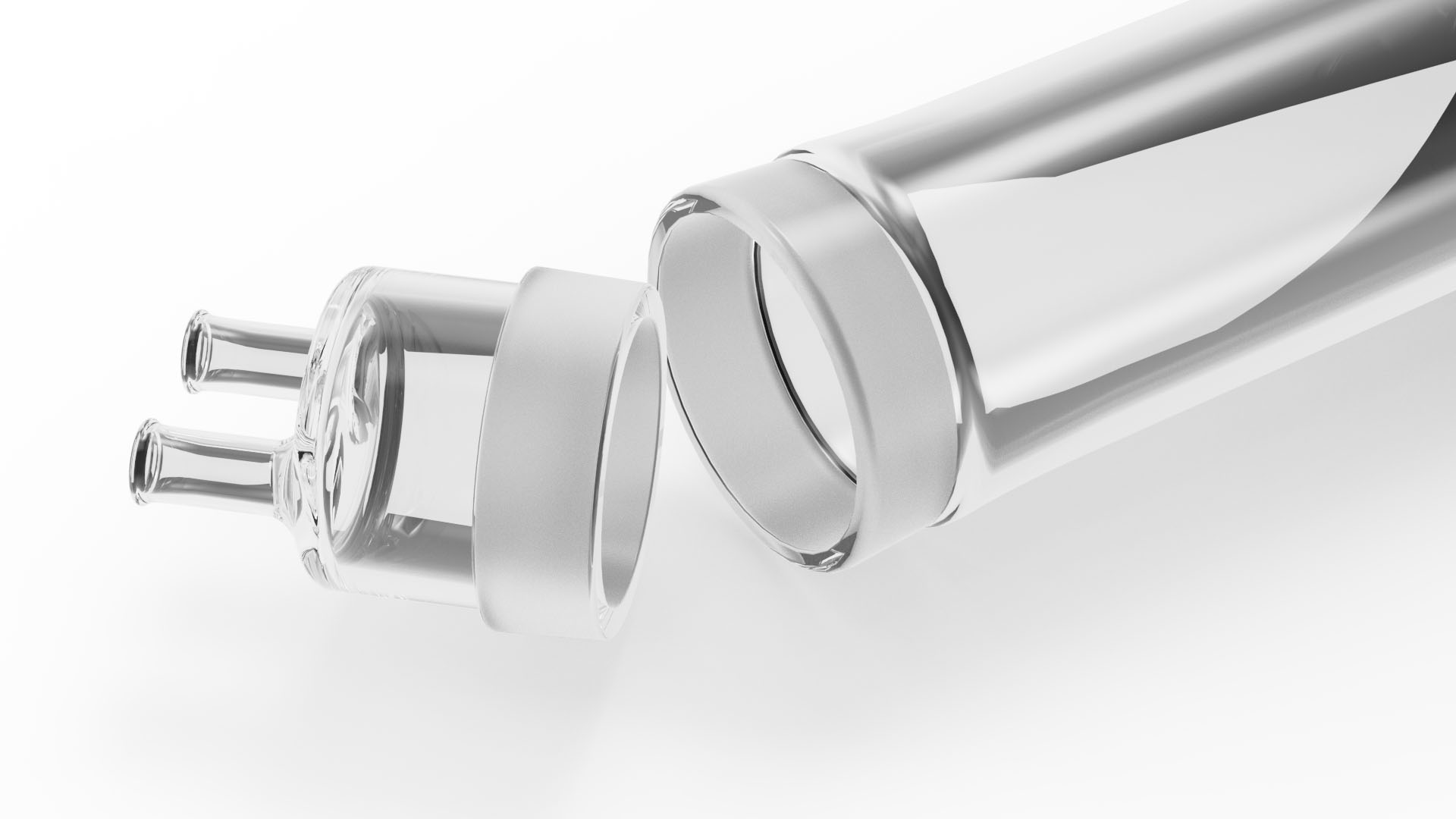
A special technique is required when working with ground glass joints. The stopper must be inserted/removed with a twist rather than a straight pull/push.
Also, when using equipment with ground glass joints, each standard taper ground glass joint should be lightly greased with stopcock grease to ensure that the joints do not "freeze" together.
Even if ground glass joints seal well without the use of lubricants, it is advisable to lubricate them to prevent sticking and breakage. Applying non-toxic silicone (stopcock) grease will help prevent that the two parts “freeze” together.
The grease should be used only sparingly by applying thin streaks to the top (wider) half of the male joint and then seat the joint by rotating gently.
Do not apply too much grease and make sure that the grease does not spread into the chamber beyond the area of the joint, otherwise the grease can dissolved in the water and contaminate your sample.
How to grease ground glass joints:
Where to buy stopcock grease:
LinkHow to find the offset temperature?
Quick reference – Finding the right temperature offset
Minute volumes of blood sample require incoming gas with a relative humidity close to 100%, to prevent desiccation or condensation. The BOBS™ instrument regulates gas humidity by modifying the temperature of the gas humidifier independently from the sample holder. To find the optimal temperature offset between the gas humidifier and the sample holder at your experimental temperature, follow the below steps.
- Power on the BOBS™ instrument and allow to warm-up for about 1-2 hours.
- Load a sample or water droplet onto the sample holder, using the same volume as for the final experiment.
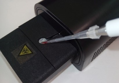
NOTE: If you are not using the pH-sensor, the entrance port for the pH sensor inside the sample holder must be covered with a small piece of tape to avoid air draft and any condensation forming inside the pH sensor tube to run back into your sample and dilute it. - Insert the sample holder and screw it tightly in place.
- Go to the main menu and select ´Experiment´.
- Set the desired experimental temperature (1) and an approximate starting offset temperature (2, see table for recommended offset values to start with).
|
Sample temperature [°C] |
Humidifier temperature [°C] |
Offset [°C] |
|
20 |
20 |
0,0 |
|
37 |
39 |
2.0 |
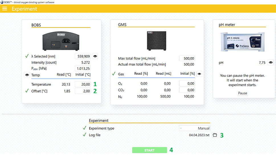
- Select the log file (3) and start an experiment (4). Ensure gas is turned on and at full flow but NOT exceeding 500 ml/min.
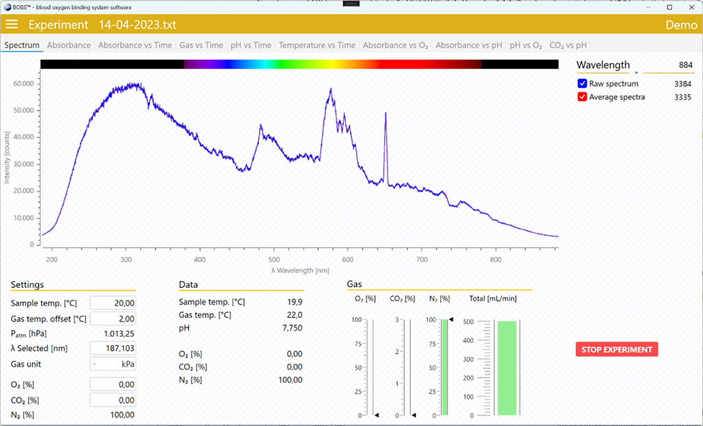
- In the “Spectrum” tab select a wavelength at which you will monitor your absorbance.
- Go to the “Absorbance vs time” tab and monitor the absorbance for about 10-15 min.
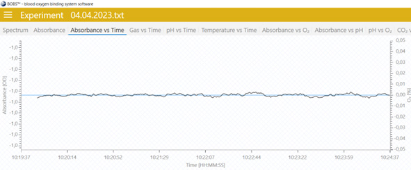
- If the absorbance does not significantly change, the sample is stable and neither dries up or collects condense water. In this case you are ready to go. Continue with step 12.
- If the absorbance:
- Increases: the sample likely collects water, which reduces the light transmission. In this case decrease the offset temperature by about 0.5°C to reduce the humidity of the incoming gas
- Decreases: the sample likely dries out, which reduces the sample droplet thickness and causes the light transmission to increase. In this case increase the offset temperature by about 0.5°C to increase the humidity of the incoming gas.
- Increases: the sample likely collects water, which reduces the light transmission. In this case decrease the offset temperature by about 0.5°C to reduce the humidity of the incoming gas
- Keep adjusting the temperature offset till you reach a stable absorbance for about 10-15 min, or for the same time as you will run your actual experiment. You may also fine-tune the temperature offset in <0.5°C.
- Stop the temperature offset experiment and use the determined temperature offset for your actual experiment run at the identical experimental temperature and conditions.
AutoResp™ v3 – Analysis - Chart settings
General
Applies to multiple graphs.
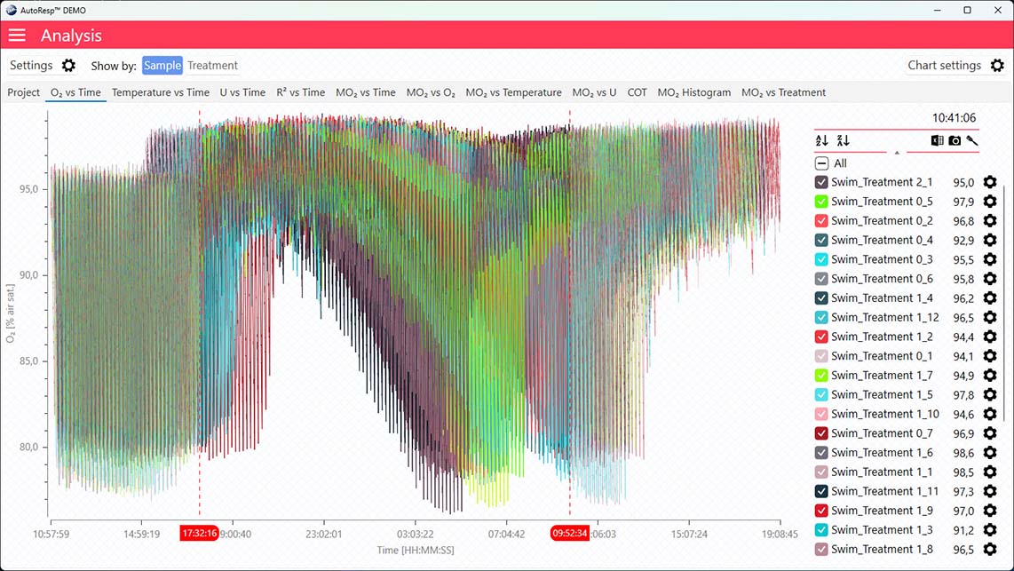
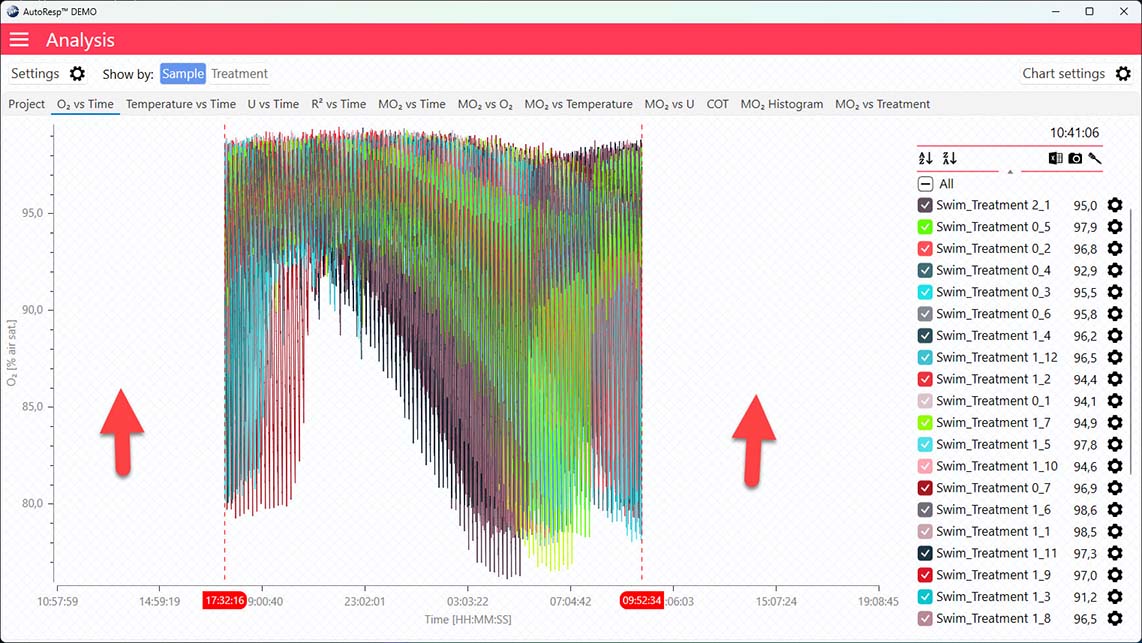
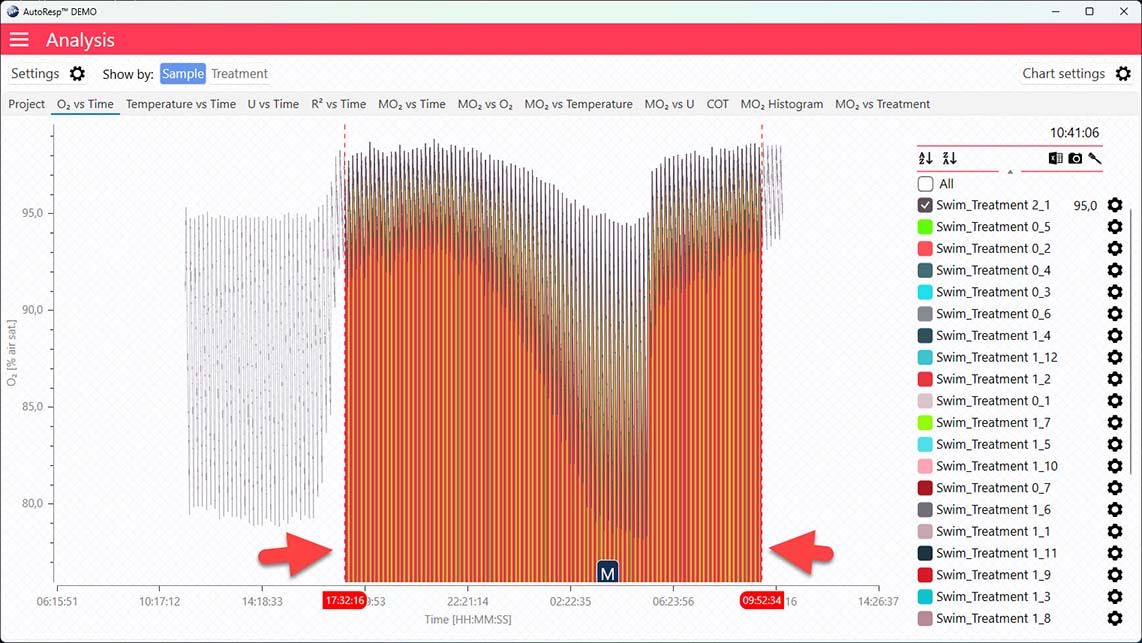
Show excluded data
Show/Hide the data displayed outside the global (or individual) date time handlers (red dotted lines). Is visible when one and multiple channels are selected.
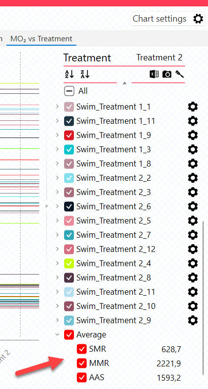
Show average
Show/Hide the average of the following calculated parameters:
SMR + MMR + AAS + Ucrit + Uopt + COTopt
These parameters can also be shown/hidden using the legend menu, when available:
Show global date time handlers
Show/Hide the global date time handlers (red dotted lines). Data outside these lines are shaded (or hidden) and not included in the analysis. Is visible when one and multiple channels are selected.
If the data range has been narrowed even further using the individual data ranges in the settings menu for that channel, the global date time handlers will not show the actual data range:
Show confidence interval
Show/Hide the confidence interval on a graph. Is visible when a single channel is selected.
Show Uopt line
Show/Hide the Uopt line. The Uopt line is available on the COT and MO2 vs U graphs. Is visible when a single channel is selected.
Show COTopt line
Show/Hide the COTopt line. The COTopt line can also be shown or hidden using the legend menu. Is visible when one and multiple channels are selected.
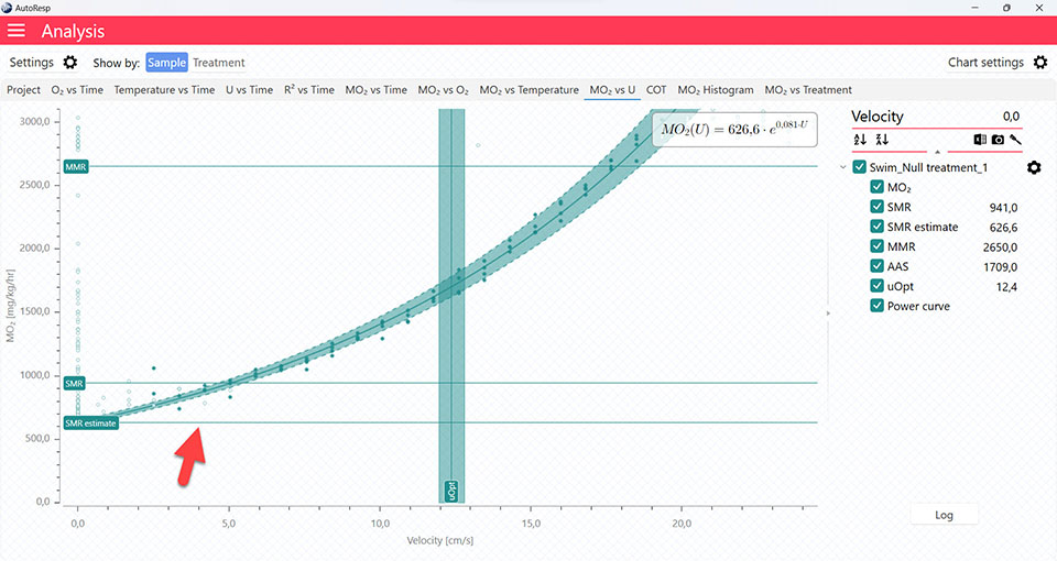
Show SMR estimate from speed curve
Show/Hide the SMR estimate based on the speed curve. Is visible when one and multiple channels are selected.
Show equations
Show/Hide the MO2 equation for the specific data graph. Is visible when a single channel is selected.
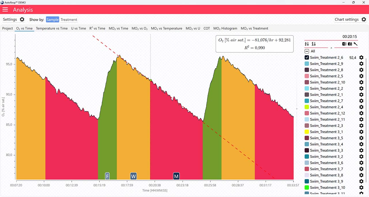
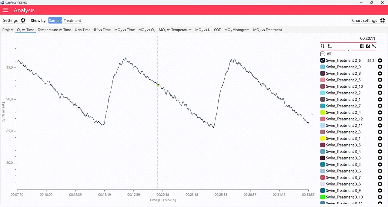
O2 vs Time
Applies to the O2 vs Time graph.
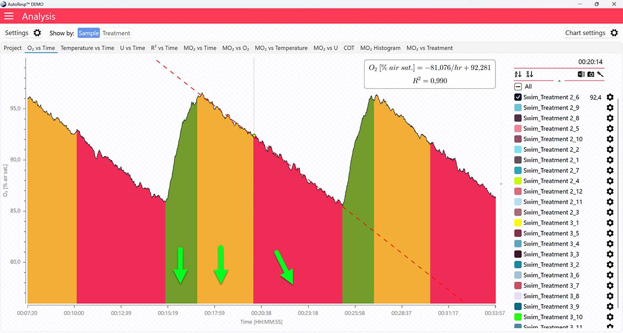
The following parameters: FWM (Flush, Wait, Measure phase), regression line, and single mode are only visible when a single channel is selected. If set to YES, the data graph for a single channel will show as:
Show FWM
If set to NO, the flush, wait, and measure indicators will not be visible.
Show regression line
If set to NO, the regression line and its equation will not be visible.

Single mode
If set to NO, the FWM phase colors will not be visible.
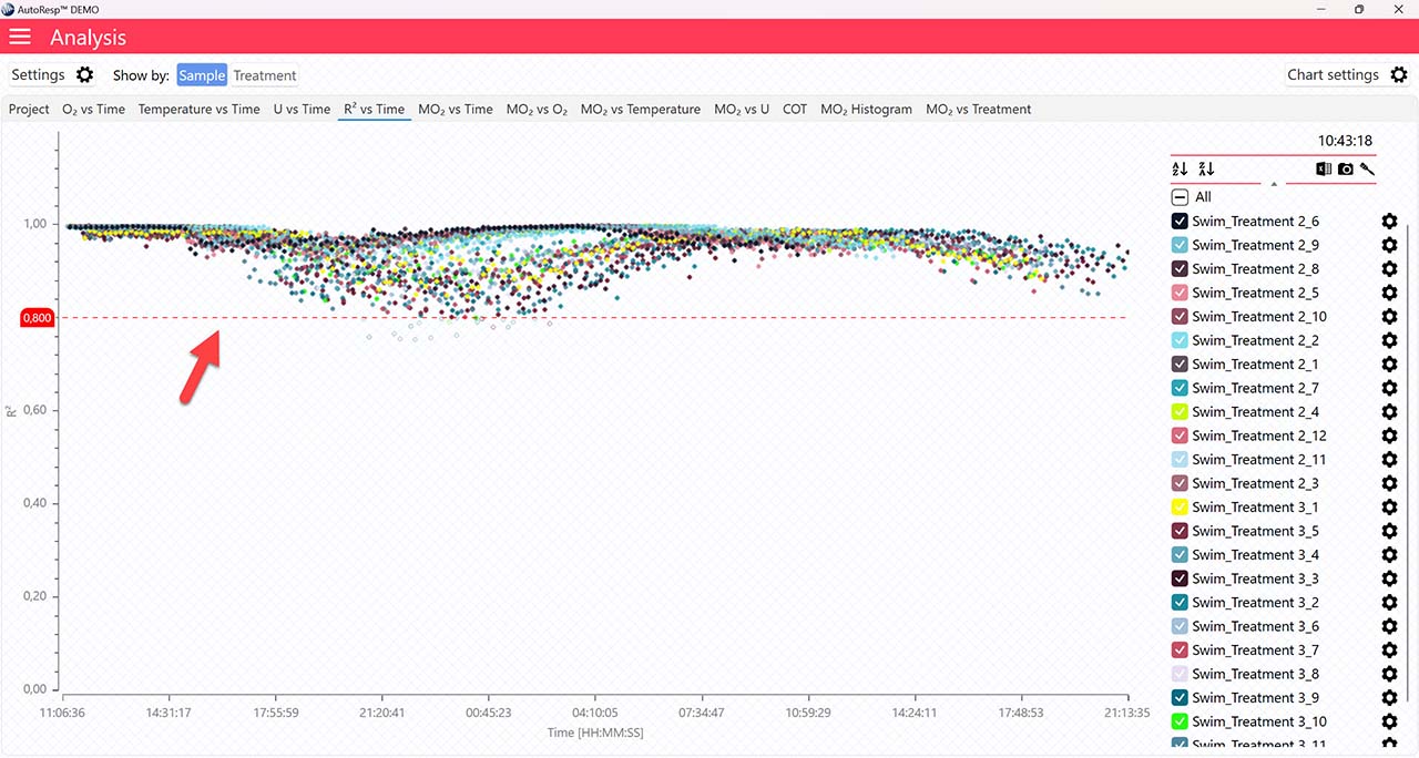
R2 vs Time
Applies to the R2 vs Time graph.
Show R2 minimum line
Show/Hide the minimum R2 value. The minimum R2 value must be specified in the Settings menu first. Is visible when one and multiple channels are selected.
MO2 vs O2
Applies to the R2 vs Time graph.
Show Min Max O2 handlers
Show/Hide the minimum and maximum O2 handlers for SMR and MMR (red dotted lines) and Pcrit (blue dotted lines). The handle values can be set in the Settings menu or by clicking and dragging on the dotted lines directly on the graph. Are visible when one and multiple channels are selected.
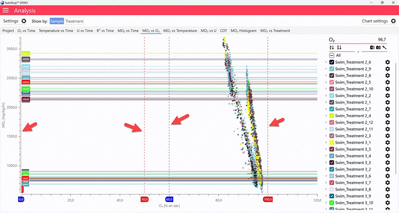
Show Pcrit value line
Show/Hide the calculated Pcrit value line based on the chosen method in the Settings menu. Is visible when one and multiple channels are selected. The Pcrit value can also be shown or hidden in the legend menu for each channel.
Show Pcrit line
Show/Hide the calculated Pcrit line based on the chosen method in the Settings menu. Is visible when one and multiple channels are selected. The Pcrit value can also be shown or hidden in the legend menu for each channel.
MO2 vs X
Applies to all MO2 vs… graphs.
Show SMR line
Show/Hide the SMR lines. Is visible when one and multiple channels are selected.
Show MMR line
Show/Hide the MMR lines. Is visible when one and multiple channels are selected.
MO2 Histogram
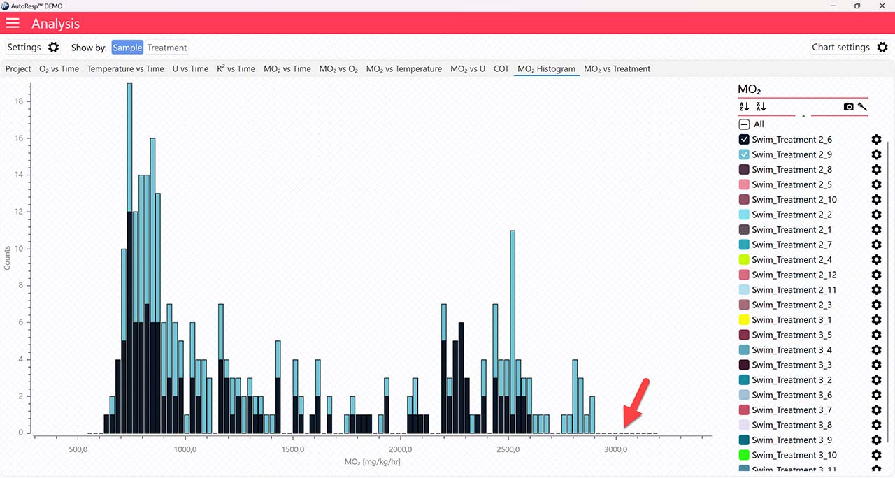
Applies to the MO2 Histogram.
Draw zero data points
Show/Hide the histogram data points that have had no counts. Is visible when one and multiple channels are selected.
AutoResp™ v3 – How to find the Standard Metabolic Rate (SMR)
Use AutoResp™ v3 to calculate Standard Metabolic Rate (SMR) from your logged data files.
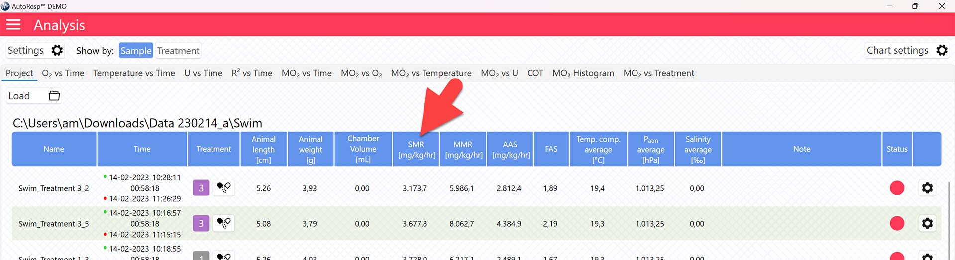
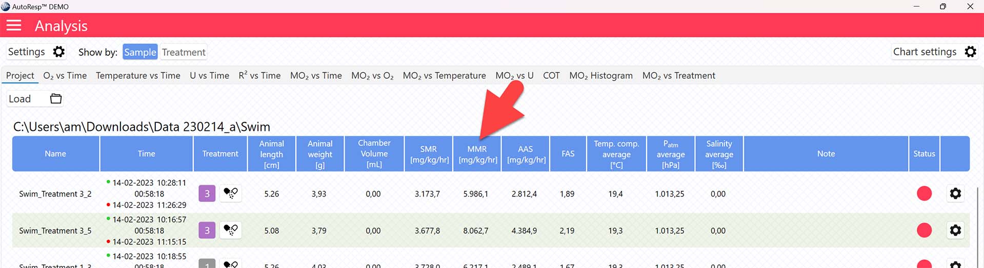
Main menu > Analysis > Project tab > Load a swim tunnel or resting chamber file (.ar3)
The SMR value is now shown in the SMR column in the Project tab for each swim tunnel or resting chamber, but note that the method for calculating SMR can be changed (see Selecting SMR-method):
Selecting SMR-method
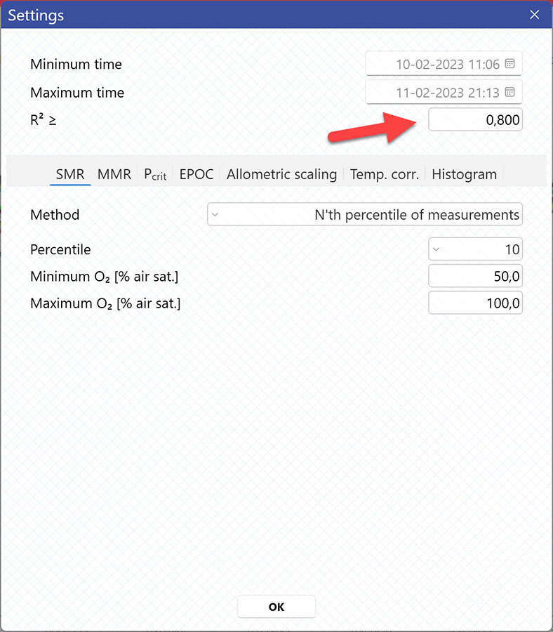
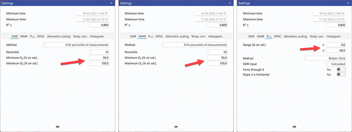
AutoResp™ v3 offers several ways of calculating SMR. The calculation method can be changed in the Settings menu > SMR tab > Method:
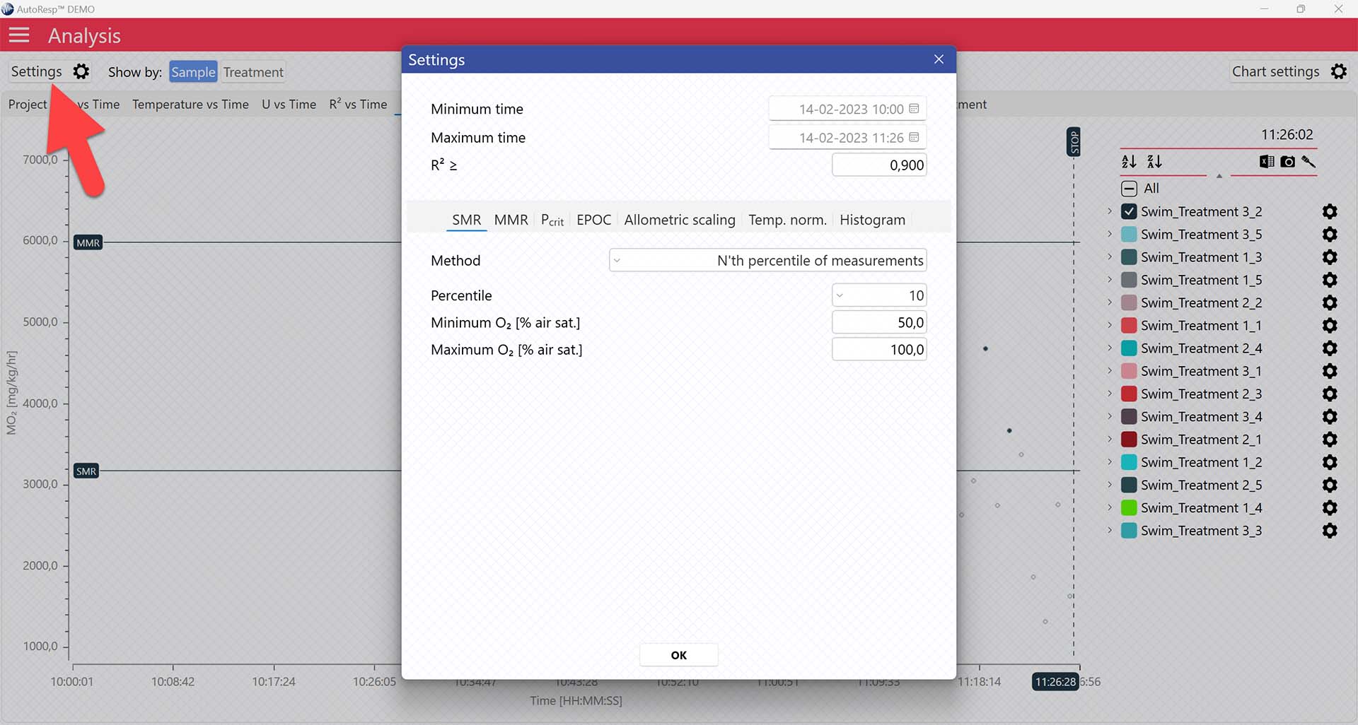
Each method is described in details in the AutoResp™ 3 - Algorithms summary.
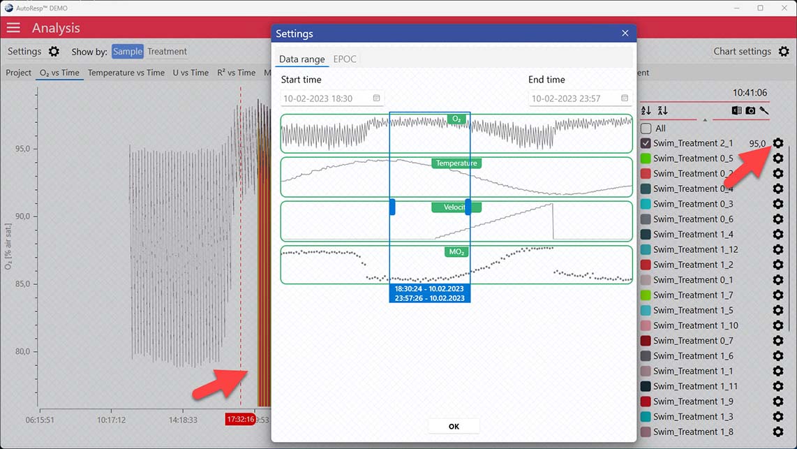
Setting data range for SMR calculations
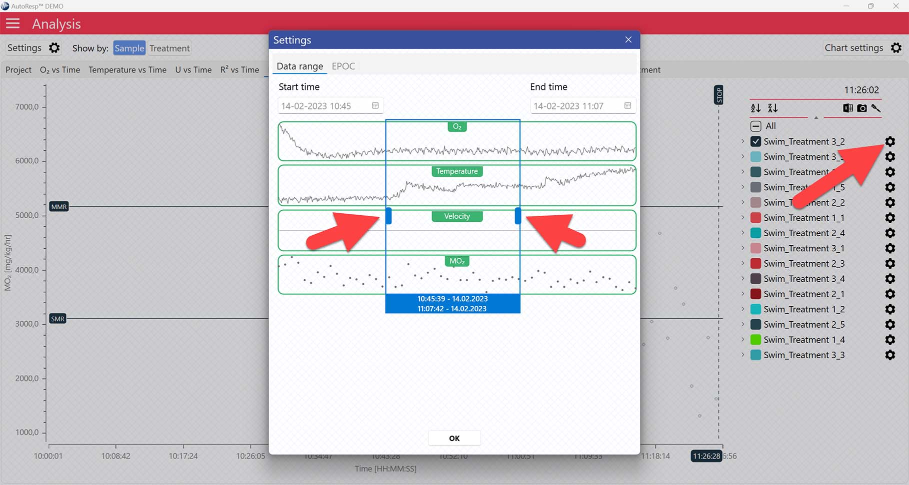
Setting a Minimum O2 and Maximum O2 value will filter away MO2-values outside the selected range, and those MO2-values will not be used in the calculations. You can also exclude MO2-values for each individual channel using the settings icon in the legend panel. Drag the blue handlers to set the range or input the values directly in the Start time and End time fields above:
A global data range (meaning it applies to all your analyzed data files) can be set in the Settings menu. Set the desired time interval or exclude data based on the R2-value:

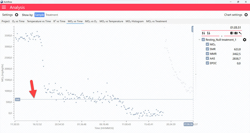
SMR graphs
The MO2 vs Time and MO2 vs O2 tabs will give you graphs with a horizontal line representing the SMR value calculated by the AutoResp™ 3. The exact SMR value is shown in the legend panel, when you open the channel using the small arrow next to the colored checkbox. Note that multiple SMR lines can be shown by selecting more channels in the legend panel:
AutoResp™ v3 – How to find the Maximum Metabolic Rate (MMR)
Use AutoResp™ v3 to calculate Maximum Metabolic Rate (MMR) from your logged data files.
Main menu > Analysis > Project tab > Load a swim tunnel or resting chamber file (.ar3)
The MMR value is now shown in the MMR column in the Project tab for each swim tunnel or resting chamber, but note that the method for calculating MMR can be changed (see Selecting MMR-method):
Selecting MMR-method
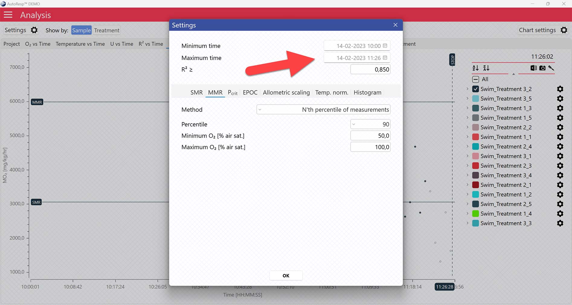
AutoResp™ v3 offers several ways of calculating MMR. The calculation method can be changed in the Settings menu > MMR tab > Method:
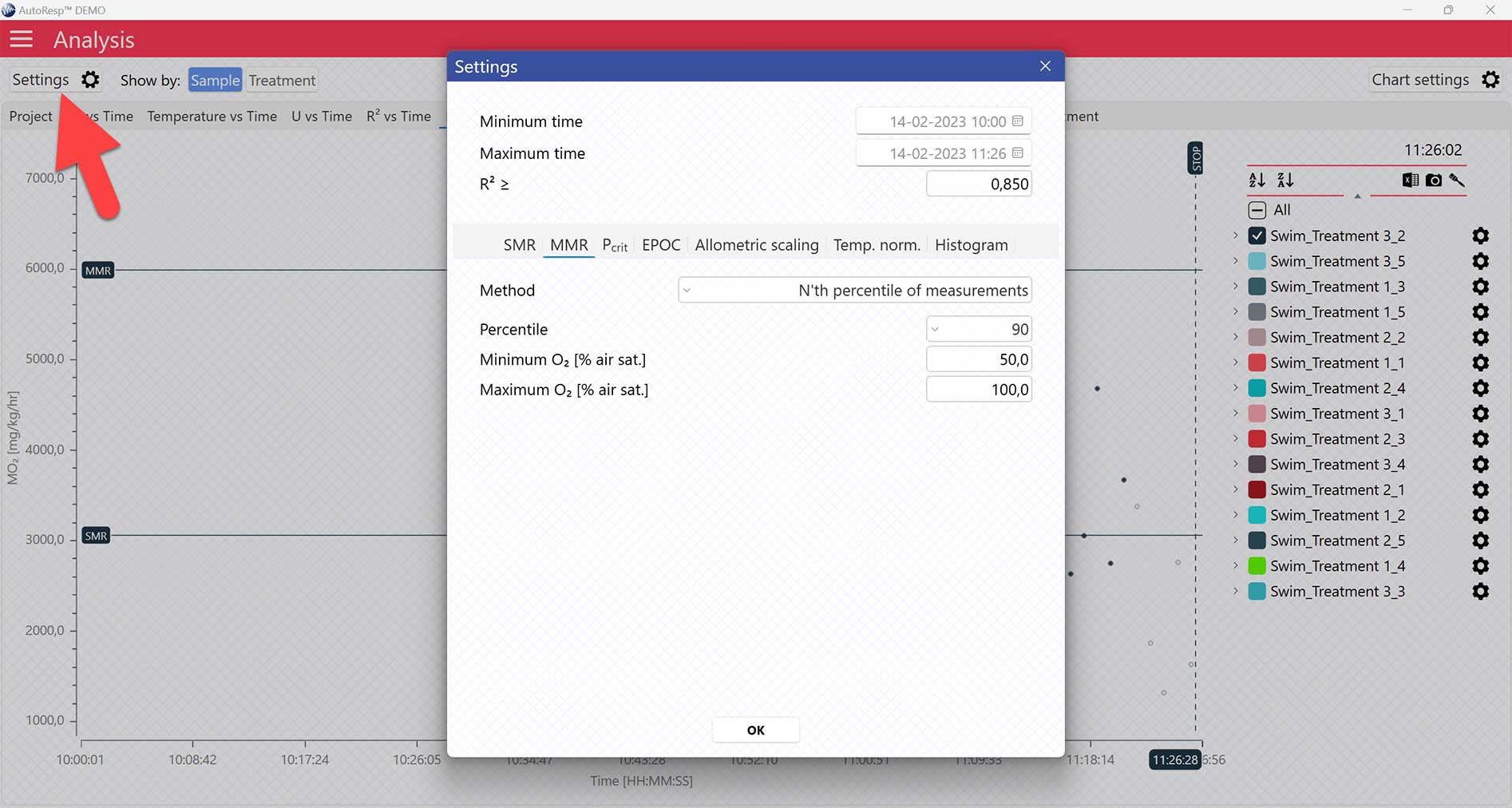
Each method is described in details in the AutoResp™ 3 - Algorithms summary.
Setting data range for MMR calculations
Setting a Minimum O2 and Maximum O2 value will filter away MO2-values outside the selected range, and those MO2-values will not be used in the calculations. You can also exclude MO2-values for each individual channel using the settings icon in the legend panel. Drag the blue handlers to set the range or input the values directly in the Start time and End time fields above:
A global data range (meaning it applies to all your analyzed data files) can be set in the Settings menu. Set the desired time interval or exclude data based on the R2-value:
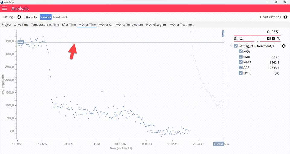
MMR graphs
The MO2 vs Time and MO2 vs O2 tabs will give you graphs with a horizontal line representing the MMR value calculated by the AutoResp™ 3. The exact MMR value is shown in the legend panel, when you open the channel using the small arrow next to the colored checkbox. Note that multiple MMR lines can be shown by selecting more channels in the legend panel:
AutoResp™ v3 – How to find the critical lower oxygen level (Pcrit)
Use AutoResp™ v3 to calculate the partial pressure of oxygen (Pcrit) below which the animal can no longer maintain a stable metabolic rate (MO2) from your logged data files:
Main menu > Analysis > Project tab > Load a swim tunnel or resting chamber .ar3 file
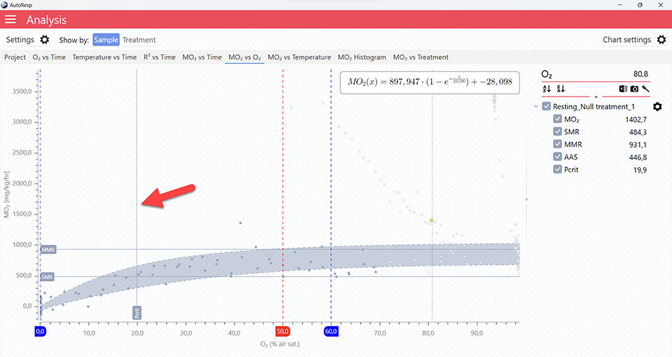
Pcrit graphs
The MO2 vs O2 tab will give you a graph of Pcrit. The exact Pcrit-value is shown in the legend panel, when you open the channel using the small arrow next to the colored checkbox.
The Pcrit value line shows where Pcrit is located on the X-axis. Note that multiple Pcrit value lines can be shown by selecting more channels in the legend panel:
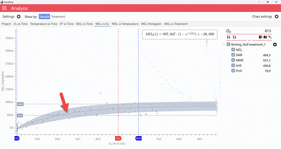
The Pcrit line shows the fitted function for the Pcrit-calculation. The colored band above and below the function is the confidence interval. Multiple Pcrit lines can be viewed by selecting multiple channels in the legend panel, but if you want to see the confidence interval for a specific Pcrit line, only a single channel must be selected:
The Pcrit value line, Pcrit line, and confidence interval can be shown or hidden using the Chart settings menu.
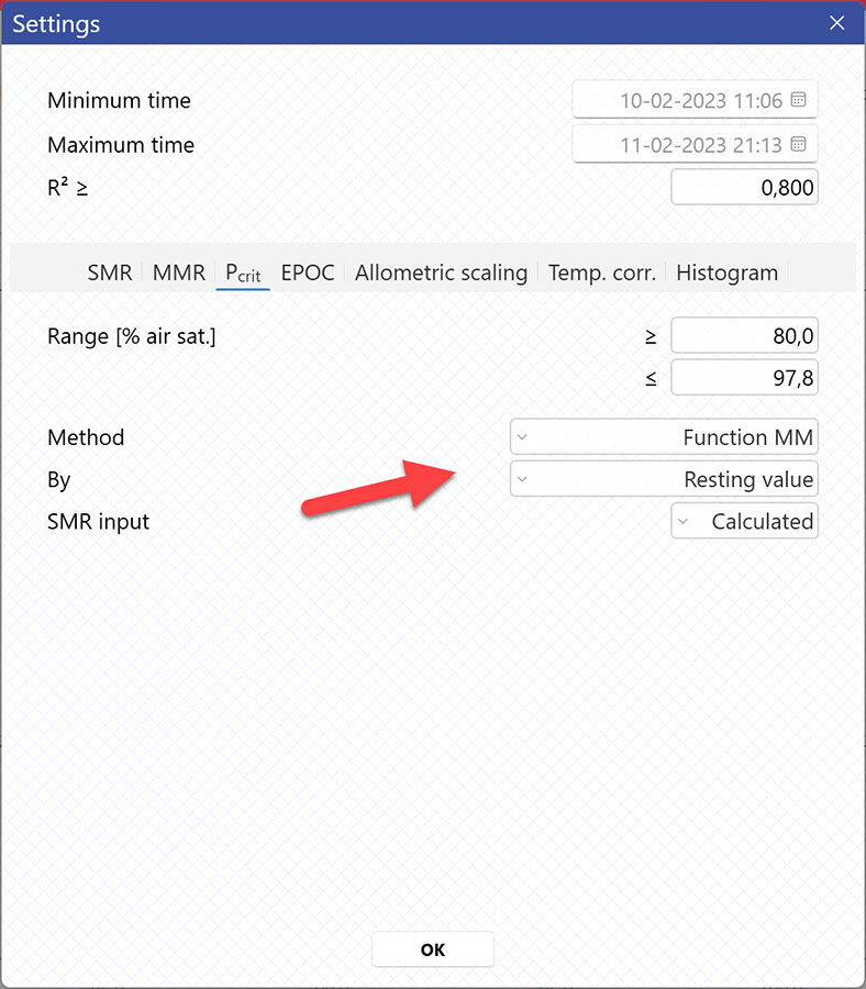
Selecting Pcrit-method
AutoResp™ v3 offers several ways of calculating Pcrit. The calculation method can be changed in the Settings menu > Pcrit tab > Method:
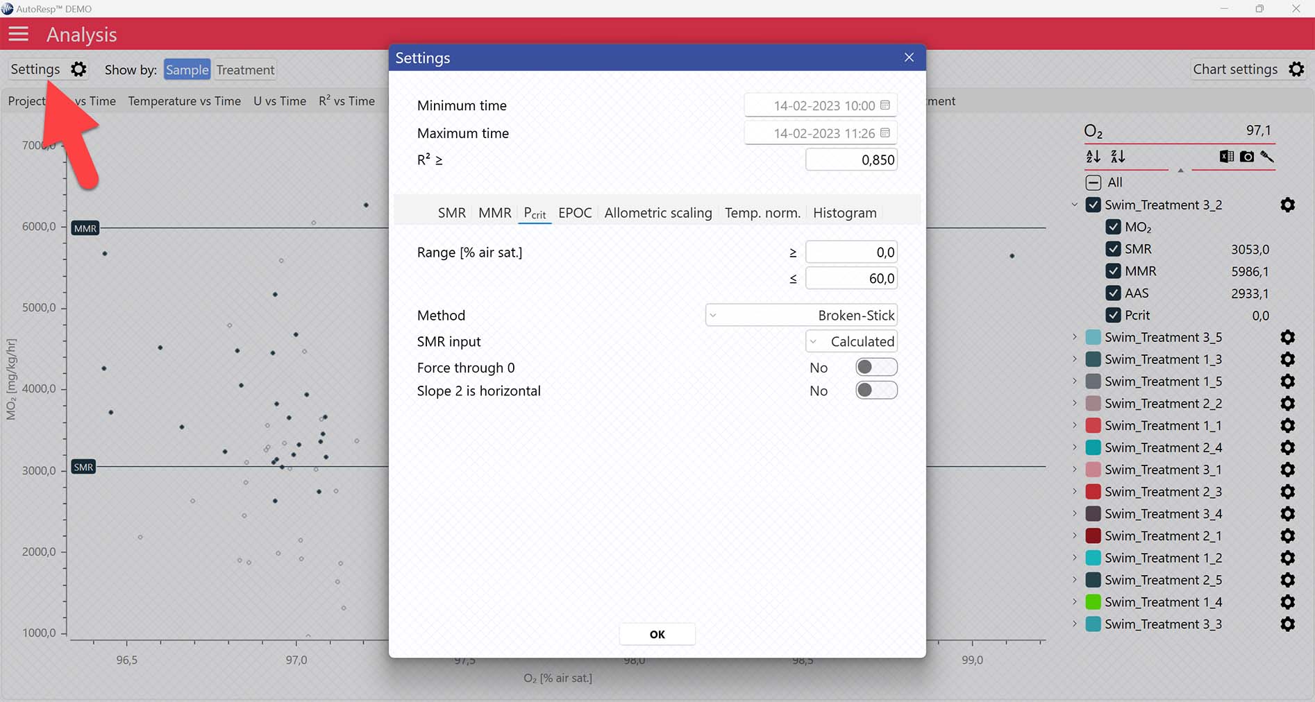
Each method is described in details in the AutoResp™ 3 - Algorithms summary.
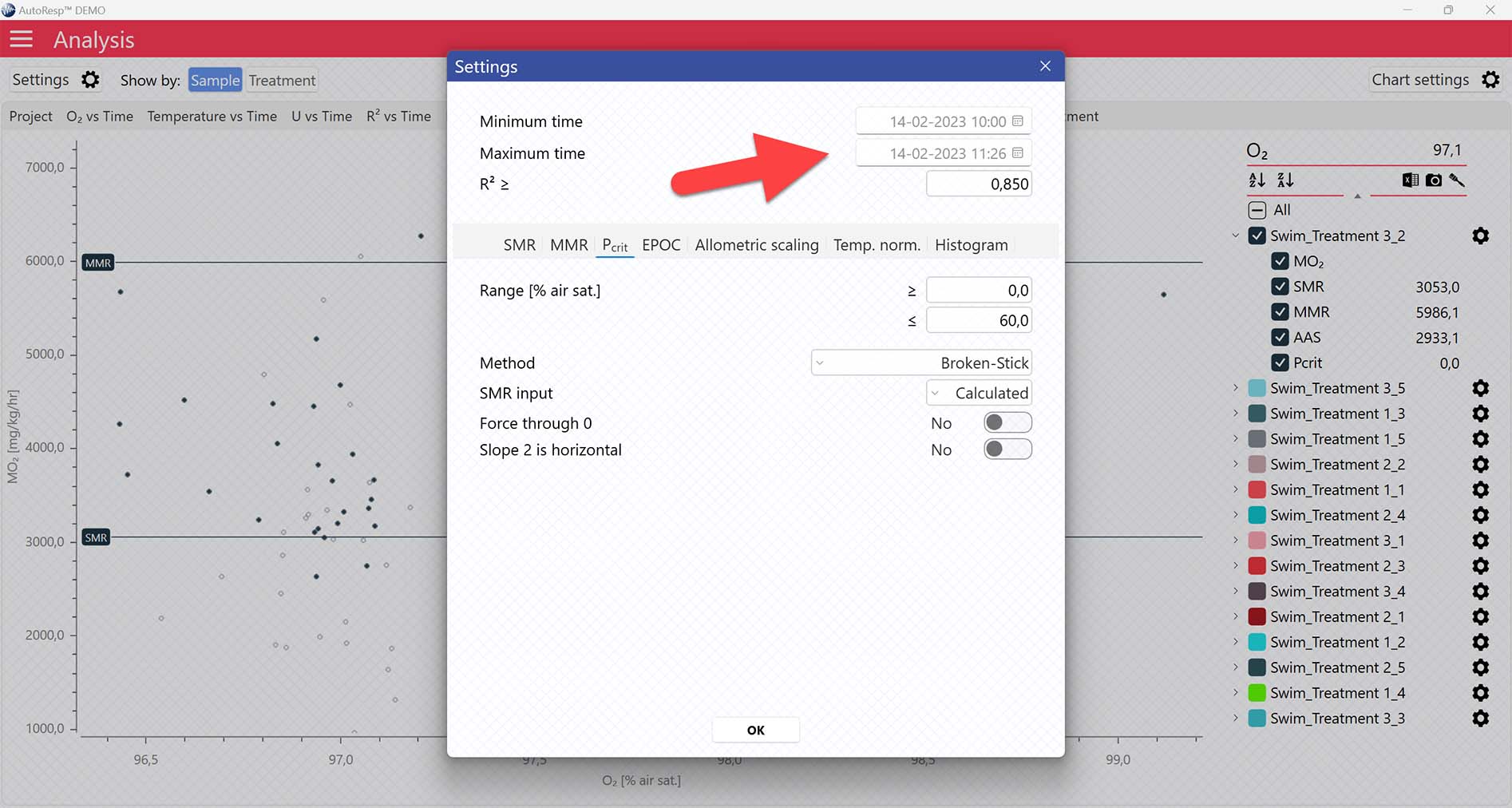
Setting data range for Pcrit calculations
Setting Range [% air sat.] values in the Settings menu > Pcrit tab will filter away MO2-values outside the selected range, and those MO2-values will not be used in the calculations. You can also exclude MO2-values for each individual channel using the settings icon in the legend panel. Drag the blue handlers to set the range or input the values directly in the Start time and End time fields above:
A global data range (meaning it applies to all your analyzed data files) can be set in the Settings menu. Set the desired time interval or exclude data based on the R2-value:
AutoResp™ v3 – How to find the Cost Of Transport (COT) and COTopt
Use AutoResp™ v3 to calculate Cost Of Transport (COT) values from your logged data files:
Main menu > Analysis > Project tab > Load a swim tunnel .ar3 file
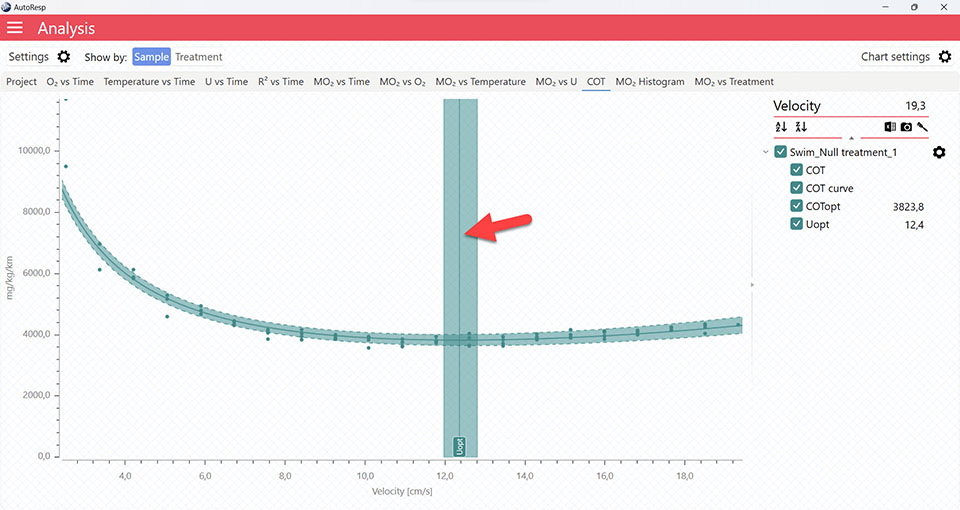
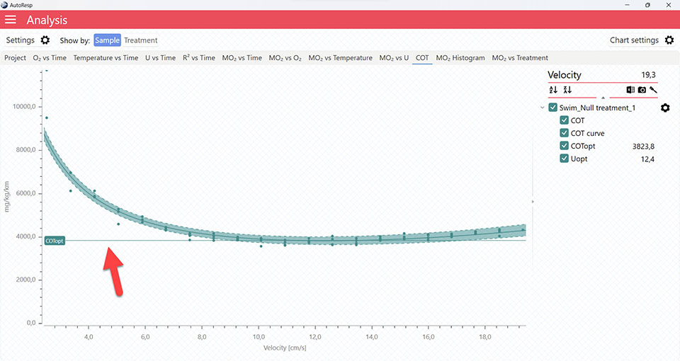
COT graphs
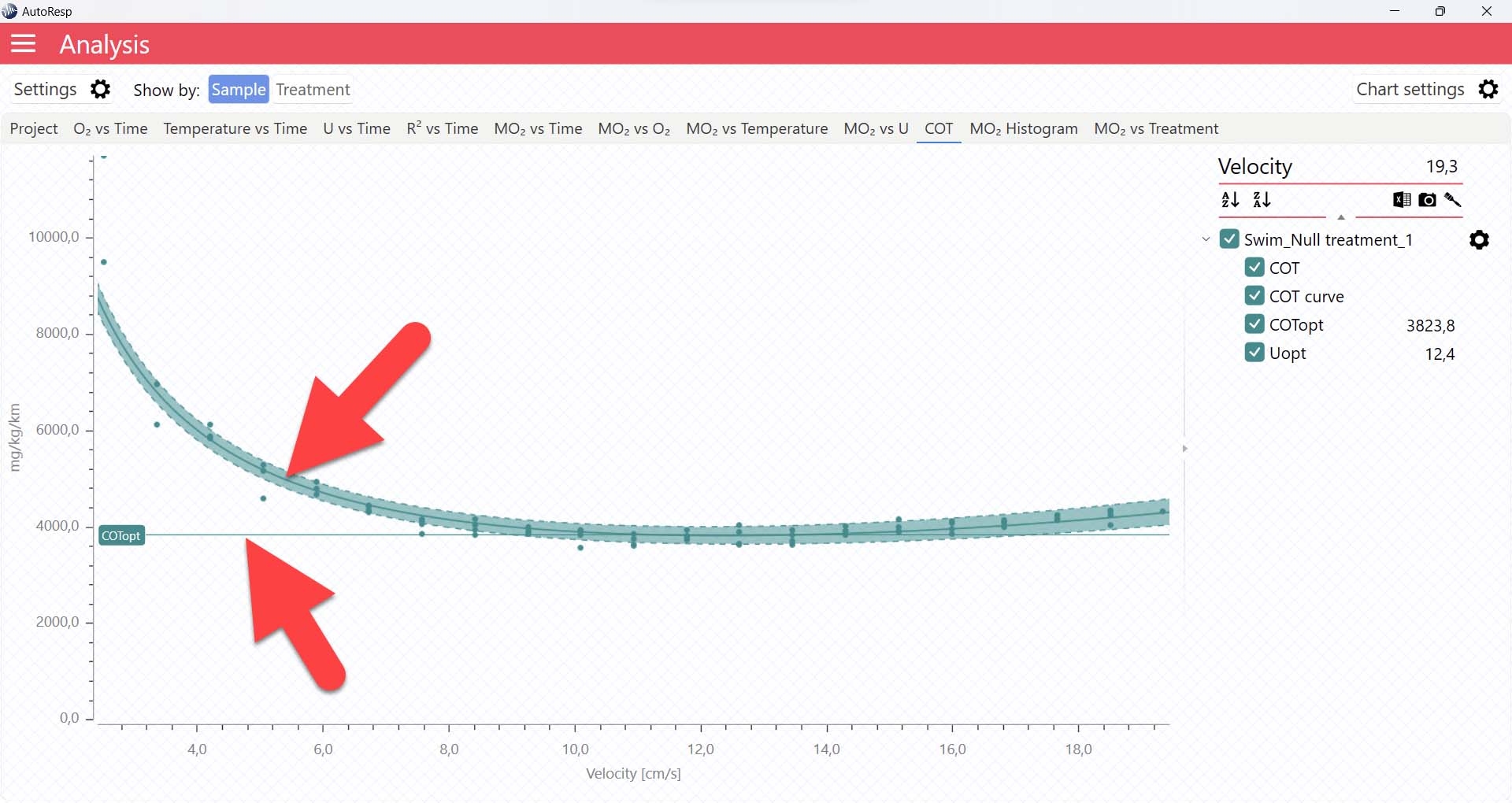
The COT tab will give you a graph of COT. The COT values are also shown in the legend panel, when you open the channel using the small arrow next to the colored checkbox. Note that multiple COTs and COTopt lines can be viewed by selecting multiple channels in the legend panel, but if you want to see the confidence interval for a specific COT or COTopt line, only a single channel must be selected:
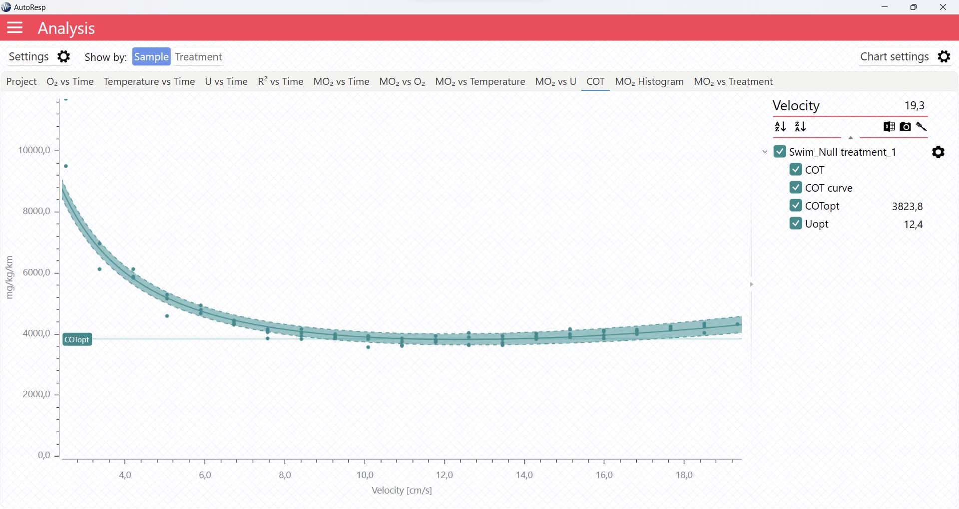
It is also in the COT tab that you can see the fitted function (COT curve) (and confidence interval, if enabled in the Chart settings menu), and the COTopt line and value. The COTopt is the COT value at the Optimal Swim Speed (Uopt):
The COT algorithms
For more details on the COT algorithms used in AutoResp™ v3, see the AutoResp™ 3 - Algorithms summary.
Setting data range for COT calculations
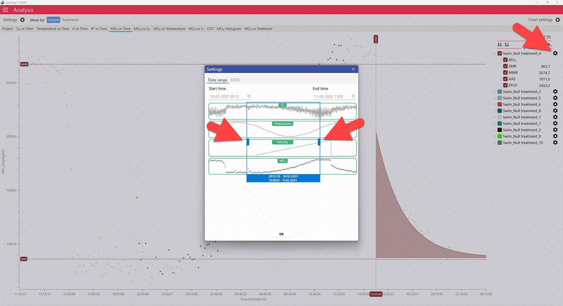
You can exclude MO2-values for each individual channel using the settings icon in the legend panel. Drag the blue handlers to set the range or input the values directly in the Start time and End time fields above:
A global data range (meaning it applies to all your analyzed data files) can be set in the Settings menu. Set the desired time interval or exclude data based on the R2-value:
AutoResp™ v3 – How to find the Optimal Swim Speed (Uopt)
Use AutoResp™ v3 to calculate Optimal Swim Speed (Uopt) values from your logged data files:
Main menu > Analysis > Project tab > Load a swim tunnel .ar3 file
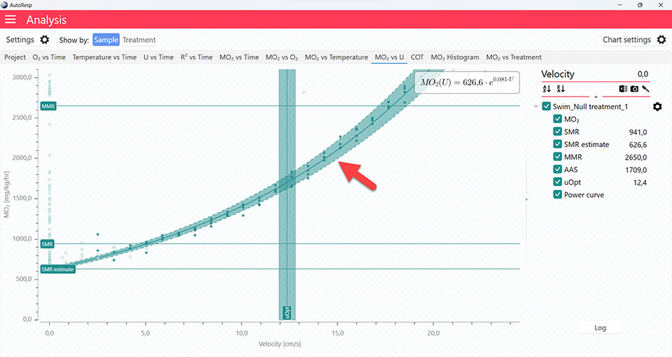
Uopt graph
The COT and MO2 vs U tabs will give you graphs with a vertical line representing the Uopt line. The Uopt value is also shown in the legend panel, when you open the channel using the small arrow next to the colored checkbox. Multiple Uopt lines can be viewed by selecting multiple channels in the legend panel, but if you want to see the confidence interval for a specific Uopt line, only a single channel must be selected:
The Uopt algorithms
For more details on the Uopt algorithms used in AutoResp™ v3, see the AutoResp™ 3 - Algorithms summary.
Setting data range for Uopt calculations
You can exclude MO2-values for each individual channel using the settings icon in the legend panel. Drag the blue handlers to set the range or input the values directly in the Start time and End time fields above:
A global data range (meaning it applies to all your analyzed data files) can be set in the Settings menu. Set the desired time interval or exclude data based on the R2-value:
AutoResp™ v3 – How to find the Excessive Post-exercise Oxygen (EPOC)
Use AutoResp™ v3 to calculate Excessive Post-exercise Oxygen (EPOC) values from your logged data files:
Main menu > Analysis > Project tab > Load a swim tunnel or resting chamber .ar3 file
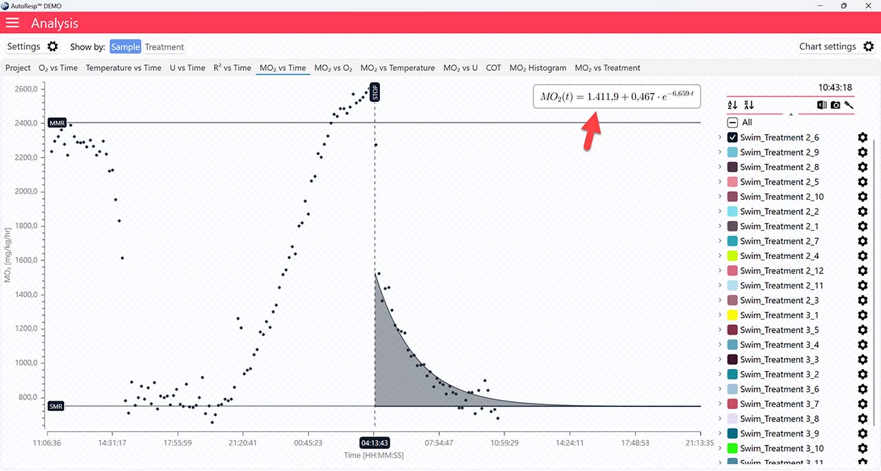
EPOC graph
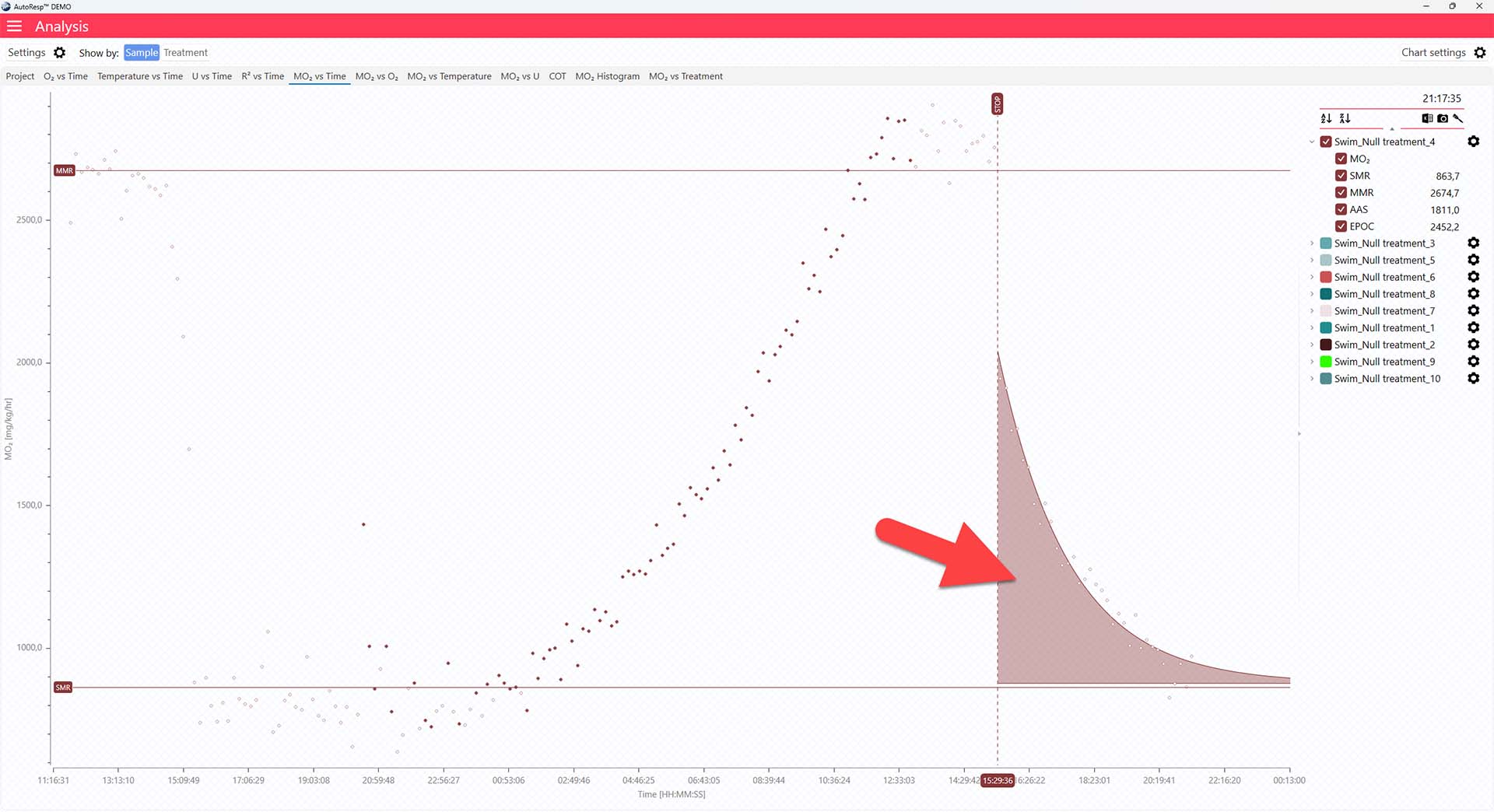
The MO2 vs Time tab will give you a graph of EPOC as the colored area after the dotted, vertical STOP line. The EPOC value is also shown in the legend panel, when you open the channel using the small arrow next to the colored checkbox. Note that only a single EPOC area can be shown at a time:
The EPOC algorithms
You can change the method used to calculate and show the EPOC value in the Settings menu > EPOC tab. For more details on the EPOC algorithms used in AutoResp™ v3, see the AutoResp™ 3 - Algorithms summary.
Setting data range for EPOC calculations
You can exclude MO2-values for each individual channel using the settings icon in the legend panel. Drag the blue handlers to set the range or input the values directly in the Start time and End time fields above:
A global data range (meaning it applies to all your analyzed data files) can be set in the Settings menu. Set the desired time interval or exclude data based on the R2-value:
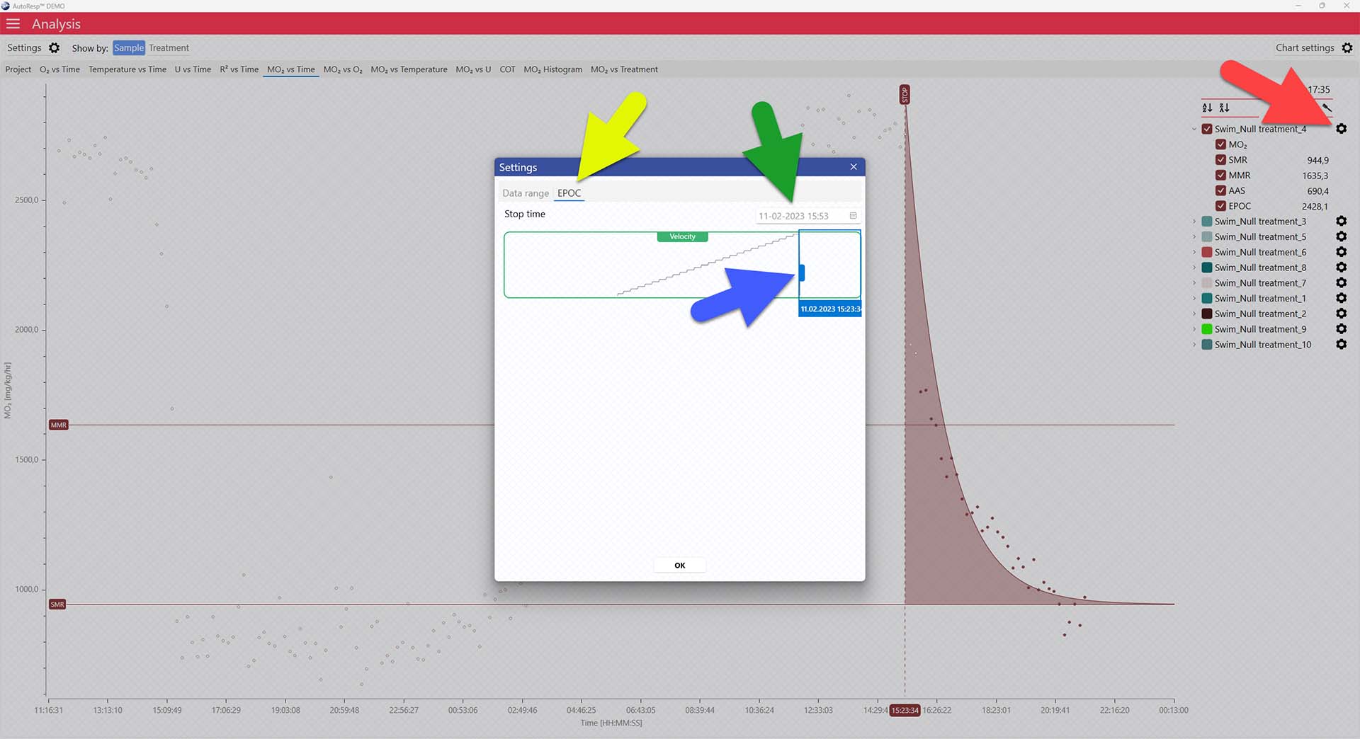
The dotted STOP line can be adjusted via the settings icon in the legend panel for each channel (red arrow). Open the EPOC tab (yellow arrow) and click og drag the blue handle (blue arrow) to place the stop value. The exact STOP line value can also be typed in using the Stop time field (green arrow):
AutoResp™ v3 – How to normalize MO2 to a specific weight (allometric scaling)
Use AutoResp™ v3 to normalize MO2 values to a specific weight (allometric scaling) from your logged data files:
Main menu > Analysis > Project tab > Load a swim tunnel or resting chamber .ar3 file
In the Project tab, open the Settings menu > Allometric scaling tab > Set enable to yes
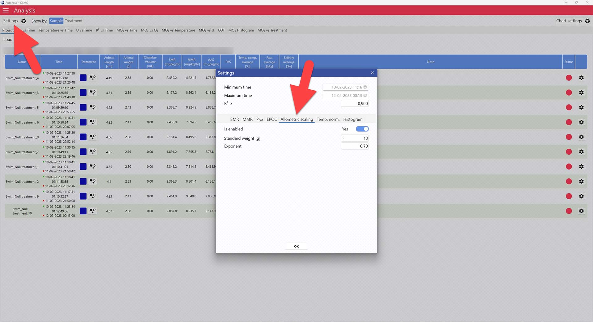
Now adjust the standard weight you want to normalize to, and change the exponent, if necessary, in the parameters below.
The allometric scaling algorithms
For more details on the allometric scaling algorithms used in AutoResp™ v3, see the AutoResp™ 3 - Algorithms summary.
LinkAutoResp™ v3 – How to normalize MO2 to a specific temperature (Temp.norm.)
Use AutoResp™ v3 to normalize MO2 values to a specific temperature (Tempnorm) from your logged data files:
Main menu > Analysis > Project tab > Load a swim tunnel or resting chamber .ar3 file
In the Project tab, open the Settings menu > Temp. norm. tab > Set enable to yes
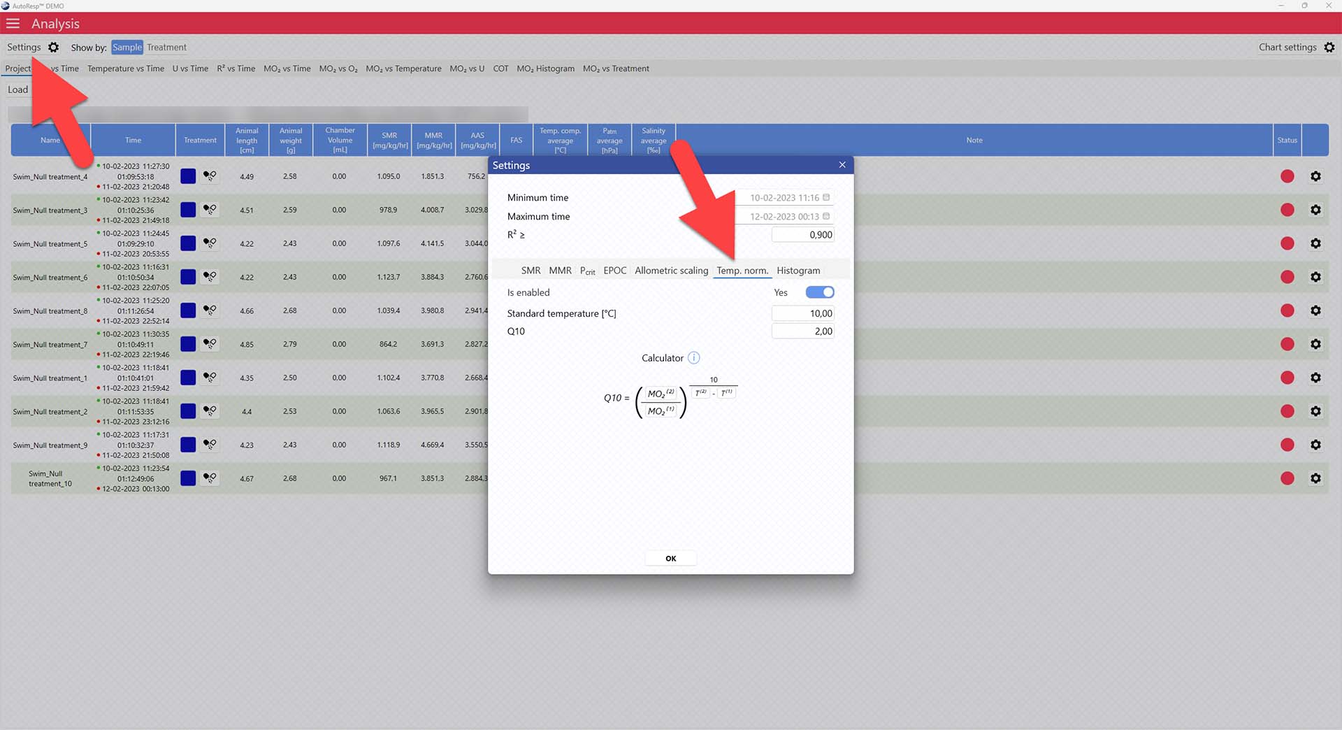
Now adjust the standard temperature you want to normalize to, and change the Q10 value, if necessary, in the parameters below. The Q10 value can be entered directly, or you can enter the individual parameters in the function below.
The Tempnorm algorithms
For more details on the Tempnorm algorithms used in AutoResp™ v3, see the AutoResp™ 3 - Algorithms summary.
LinkAmplitude and Sensor Health
Optical oxygen sensors, also known as optodes, work by emitting red fluorescence from the sensor when excited by blue light from the light source of the instrument. The intensity of this red fluorescence, known as the amplitude, can be used to assess the health of your oxygen sensor. As the amplitude decreases, the quality of the measurement deteriorates as the signal-to-noise ratio is reduced.
Amplitude naturally decreases over time through a process known as bleaching. Under proper use, these sensors can remain functional for more than a decade. However, exposure to strong UV light, such as certain indoor lighting or direct sunlight, accelerates bleaching, causing the amplitude to drop rapidly, shortening the sensor's lifespan.
For sensor spots such as PSt3 and PSt5, which are used in our resting chambers and microplates respectively, the signal amplitude is reduced when the light emitter is not positioned directly over the sensor spot. Therefore, we always recommend double-checking the alignment between the emitter and the sensor in these systems.
As a rule of thumb, when the amplitude falls below 10000, sensor readings become less reliable due to higher technical variability. We recommend changing the sensor at this point for optimal data quality.
Once the amplitude drops below 3000 the sensor should no longer be used. At this stage the reproducibility and stability of the readings cannot be trusted.
LinkMicroResp - How to get the oxygen consumption rate per volume
To get oxygen consumption rates per volume rather than per well (or organism) you turn off the “Organisms per well” in the settings section of the Experiment tab, as shown in the picture below, the software will then calculate the MO2 based on the Well volume you set in the same section.

To select the preferred MO2 unit, go to the Settings tab in the Analysis section, which is shown in the image below, here you find the new MO2 units per volume by clicking on the dropdown menu and selecting your preferred unit.

Link
AutoResp™ v3 – How to apply solid blocking correction
What is solid blocking
In a closed swim tunnel a solid object will change the velocity of the flowing water. This effect is known as solid blocking, which is something we can compensate for based on the work by Bell, W.H. & Terhune, L.D.B. (1970).
The full formula can be found in the Autoresp 3 - Algorithms summary (link)
In brief, the formula works by calculating a correction factor based on a number of parameters:
- Length of the fish
- Radius of the fish
- Shape of the fish
- Cross-sectional area of the fish
- Cross-sectional area of the swim tunnel
Taken together, we can calculate a fractional error which we can multiply the measured swim speed by to get the corrected swimming speed.
In Autoresp, the fractional error can be applied in two ways: you can enter it manually, or you can have Autoresp compute it automatically using your fish’s measurements.
Autoresp then uses this value to correct the water velocity, i.e., it reduces the motor RPM so that the actual water velocity inside the test section matches the target swimming speed you defined for your experiment.
MicroResp - Error "No splitter found - please connect splitter with SDR"
The pop-up with the error message "No splitter found - please connect splitter with SDR" typically comes from a missing driver.
For most PCs, this driver is distributed alongside Windows updates, but in certain cases it is missing. When the driver is missing, the USB splitter cable is not recognized by Windows resulting in the error message.
To fix it, please do the following steps:
- Download the driver from this link
- Unzip and install the driver
- Restart your PC
- Try to connect again via MicroResp
Link